OpenGL 3D Graphs

Introduction

glgraph (OpenGL 3D graphing utility) was written primarily to provide stereo 3D graphing of surface functions. Initially this was to support surfaces on regularly spaced grids and it was later extended to randomly distributed data. The goal was not to create a full featured 3D presentation graphics package but rather an exploratory tool for 3D datasets.

The basic use involves running the program, loading a data file, and choosing options from the menus or keyboard commands. Note that for presentation purposes almost all the menus options can be specified as command line options. The mouse is used for most of the navigation but some actions require the keyboard, for example "+" and "-" for zooming in and out.

The data can be display in the following ways.

• Points
  Each data value is simply drawn as a single pixel.

• Wireframe
  The connectivity between points is drawn as line segments, this will be of the form of a grid for regularly spaced data or triangles for randomly distributed datasets.

• Flat shaded, Smooth shaded, Lights
  In these three modes the surface is drawn solid with varying degrees of shading quality.

• X contours, Y Contours, XY contours, Z contours
  These modes draw regularly spaced contour lines in the indicated plane.

File formats

glgraph reads two file types, both are ASCII files containing numbers separated by "white space (spaces, tabs, carriage returns, linefeeds). In addition files with viewing position parameters can be saved and loaded from the command line or menu option.

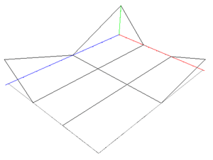
The first type of file represents a regularly spaced grid, at each point in the grid a height is known. The format is as follows, first there are two numbers specifying the number of samples in the plane, nx and ny (x and y axis). This is followed by the grid spacing of the x axis and then the y axis. This is followed by a grid of height values, there will be nx * ny of them.

A very simple example might be as follows 4 3 0 1 2 3 0 2 4 3 0 0 1 0 0 0 0 2 0 0 0

This is a grid with 4 samples in the x axis, 3 in the y axis (first line). The x grid contains values at 0, 1, 2, 3 (second line) and the y axis contains values at 0, 2, 4 (third line). Note that the layout of the numbers in this example need not be as shown, the ascii data is simply read using the C fscanf() function. The resulting graph is shown above, the x axis is in red, the y axis in blue and the z axis (height) in blue.

Random point data

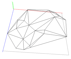
The second type of data consists of randomly distributed samples on a plane. This data can either be Delauney triangulated to form a mesh of triangular facets approximating the surface or just displayed as a point cloud. These files are simply a list of (x,y,z) triples.

0.621211 2.04291 0.50 -0.879983 -0.320499 0.40 -1.08784 2.31857 0.40 -2.9065 0.504541 0.20 -2.04379 -0.697705 0.50 1.14603 -2.64685 0.44 2.39913 -2.01872 0.36 -2.04557 0.198388 0.40 0.624865 0.496194 0.60 -1.38017 -0.657131 0.50 -1.2396 1.45426 0.50 -1.20885 -2.54677 0.40 -0.570104 2.14427 0.45 2.65181 0.976984 0.55 2.07885 -2.98347 0.20 -0.225725 0.195576 0.35 1.72726 -1.40633 0.54 2.89651 -1.15929 0.51 0.605131 0.652294 0.45 -1.72537 2.31537 0.47

Note that the Delauney triangulation results in a triangular mesh that covers the convex hull of the data points. This means that randomly distributed points that are intended to cover a concave region will

Command line

The current command line arguments can be obtained by typing "glgraph -h" (help).

Usage: glgraph [command line options]
Command line options
   -s    active stereo mode
   -ss   dual screen stereo
   -f    full screen mode
   -d    debug mode
   -z    height scale factor
   -r_   shading mode (rp, rw, rf, rs, rl)
   -og   open grid file
   -or   open random point file and triangulate
   -op   open random point file
   -vf   open view file
   -res  resolution subsampling (1,2,3,4,5)
   -h    this text

The keyboard commands are listed below, they can also be displayed on-screen with the "f1" key.

   left arrow - rotate camera left
  right arrow - rotate camera right
   down arrow - rotate camera down
     up arrow - rotate camera up
          i,k - translate camera up, down
          j,l - translate camera left, right
          -,+ - move back, move forward
          [,] - roll anticlockwise, clockwise
            h - home
1,2,3,4,5,6,7 - special camera views
            z - change height scale
            c - change contour levels
            w - write the current image to disk
            W - write a high resolution image
            D - delete geometry
        ESC,q - quit
           f1 - toggle onscreen help
           f2 - toggle stereo
           f3 - toggle image recording
           f4 - toggle construction lines
           f5 - toggle bounding box
           f6 - toggle axis display

There are a large number of features available by using the right mouse button (GLUT library standard). Some of these are listed below.

• A number of colour ramps are provided, these specify how height is mapped to colour.

• The z axis can be independently scaled, this is useful because while the x and y axes (plane) are often in related units, the z axis is often in very different units. glgraph normalises the z axis to 0->1 and then applies the zscale factor.

• For the contour rendering modes the number of contour segments can be chosen.

• While "glgraph" is intended as a data exploration tool rather than a presentation tool, it does allow screen capture. The window contents can be written to disk as a TGA image, see the "w' keyboard command.

• To assist in the interactivity of very large datasets the surface is subsampled while the user is using the mouse. The full resolution is returned when the interaction stops.