Introduction This report describes some of the computer based techniques which can be used to aid in the visualisation of terrain. In the following discussion it is assumed that we have acquired data in a suitable form which allows us to define the surface on a computer. This usually starts as a series of points lying on the surface and stored as x,y,z triples. There are many ways of getting this data, the example here was digitised from contour maps using a large scale digitising tablet connected to a computer. The next step is normally to turn the digitised data into a series of polygonally bounded planes, called facets, so that they can be read, viewed and manipulated by 3D modelling and rendering software. The point data is this example is transformed into a regular polygonal mesh by an algorithm called Delaunay triangulation See an earlier discussion by myself for details of this algorithm and computer program which transforms randomly distributed spot heights into triangular or regular meshes and exports this surface description in a format suitable for most 3D modelling and/or rendering programs. ContouringContouring has been the traditional way of presenting 3D terrain data on 2D sheets of paper. It has advantages of having units (contour values) so precise height calculations can be made. Contour lines are usually drawn with line segments so they can easily be transferred to large scale hard copy devices such as plotters. The main problem with this visualisation technique is that it does not give a good 3D impression of the terrain, the best most people can determine is that some localised parts of the surface are higher or lower than others. Mesh representationsThis is the most straightforward way of rendering the 3D data, it is a direct perspective viewing transformation of the computer database. (Almost any 3D modelling package can display, view, and print this representation, MicroStation was used here due to its advantages when handling very large geometric databases).
This rendering can also be in colour. The colour may be related to height but it could also be some other attribute such as ground cover, population, etc. The example in Figure 1 is a 128x128 cell mesh and it consists of about 33,000 line segments. On many high end computer platforms this can be drawn in real time so that the user can "fly" about the landscape. This number of polygons can however cripple many desktop machines. For this reason good terrain modelling software allows the user to view the surface at a range of resolutions. Vertical contouring
Shaded renderings Higher levels of realism can be achieved by simulating more closely how the terrain would appear in reality. There are a wide range of techniques for accomplishing this, each technique generally involves a trade off between realism and computation time.
Physical models Given the digital model it is possible to determine the path required to manufacture the surface using a computer controlled milling machine. In its simplest form this is a drill which can be controlled backward and forward and up and down over a piece of wood say, so as to cut away unwanted portions.
Figure 4 shows the result of milling our example landscape from wood. I used a OH-FANUC, model 2R-NC milling machine operated by the School of Engineering, Auckland University. The machine is controlled by the MasterCAM software For this example the wood is about 300mm square and the drill bit used in about 5mm radius. Note that it is not necessary to use a particularly fine bit because the wood is cut away at the edge of the bit not from the bottom. The bit size then only determines the narrowest valleys that are possible. This physical scale model of the landscape has big advantages for visualisation purposes. The model is to scale, although in this case there is a 2 times exaggeration in height. The viewer can instantaneously view the terrain from various positions and angles by simply turning the model about. Tactile exploration of the model is of course possible and can be informative as well as satisfying. An extension of this technique would be to automatically draw features such as roads, boundaries, contours, etc onto the landscape. This could be done with a robot arm holding a pen or with a laser which would burn the line features onto the surface of the wood.
Data reduction in terrain modellingWritten by Paul BourkeJune 1994 A common characteristic of terrain modelling/rendering exercises is the vast amount of data involved. This is particularly severe where the spot height information is a result of some automated survey or when it results from digitised contours. In addition there are a number of activities which require very different levels of detail, for example the detail required for high quality renderings may be quite high. The information that a 3D modelling package can handle while retaining user interaction may be quite low. The need for multiple terrain representations can arise naturally in modelling applications, for example it may be necessary to acquire a more course terrain model for interactive modelling and substitute a more detailed version for final presentation. As with many computer based activities there is often a gap between what one might like to and what is practical given disk, memory, or processing resources. There are two common representations for computer based terrain models. The first consists of a triangular mesh of polygons, this is normally the result from a triangulation process. One advantage of this approach is that it naturally generates detail in the regions that are sampled more frequently, these are normally the regions which have more height variation. This representation is a more faithful representation of the underlying data since the sample points are generally the vertices of the triangular mesh. The second form of representation is as a regular mesh of rectangular polygons, these are generated by estimating the heights at each corner of the mesh cells. The main advantage with this is that multiple resolution meshes can be readily generated from the same dataset of spot heights. This form is tend to provide more 3D visual cues as the wire frame rendered mesh acts a type of slope based shading. Triangulation example In this example the original digitised aerial survey resulted in 600,000 spot heights, covering a rectangular region of 42km by 64km. Converting this directly to a triangular mesh would result in a surface of approximately twice that number of polygons, 1.2million!. This number of polygons would certainly be a handful for most software packages especially if interactive 3D control was necessary. One approach to data reduction is to filter the spot heights file so as to evenly distribute the points over the region. This is done by checking the distances between all points so that no two points are closer than some user chosen distance. An improved approach would be to incorporate the height variation between neighbouring points so that highly sampled areas are better represented, this assumes that regions are densely sampled because of increased height variation. Below are some examples of the surface and the number of resulting polygons for 1,3,and 5km filter distances.
5km radius, 116 polygons 
3km radius, 316 polygons 
1km radius, 2600 polygons  Notice there are only a few polygons in the lake regions where no sampling was necessary. Gridding example This example uses another terrain database containing 100,000 points over a 650m square area. These were used to produce a gridded representation at a user selected resolution and thus file size. This very precise control of resolution is not possible in the previous filtering process, the user didn't know the resulting number of polygons beforehand. The exact size of the grid cells is also precisely known which can be useful for rough distance estimates. The following are some examples of 10, 20, and 65 square meshes showing the number of polygons involved.
10x10 grid, 65m grid size, 40 polygons 
20x20, 32.5m grid size, 200 polygons 
65x65, 1m grid, 1850 polygons 
There is normally a further overhead if a rectangular mesh surface is to be
used for rendering purposes because the 4 point facets above will generally not
be coplanar. The simplest solution is to split each facet into two along the
diagonal thus increasing the number of polygons by a factor of 2. A better
method is to interpolate the midpoint, unfortunately this increases the number
of polygons by a factor of 4.  In summary, the two representations can be used to create a terrain model of any desired data size. Indeed one would normally generate a number of surfaces with different resolution, the particular one used at any given time would depend on the applications ability, the response times, and quality/precision goals.
Terrain morphingWritten by Paul BourkeApril 2001
Source code that created the examples below. Morphing is a popular technique in the computer graphics industry extensively used in Michael Jackson videos but also used in countless movies and television ads. The technique was first used in the early 1980's, one of the first movies that used morphing was "Indiana Jones and the last Crusade". Morphing is a very different technique to fading, in that case the colour of each pixel in an intermediate frame is a linear interpolation between the colour of the corresponding pixel in the start and stop frame. For example
 In morphing one tries to capture a sense of the geometric transformations between the start and stop frame. In what follows a standard morphing technique as presented by Thaddeus Beier at the 1992 Siggraph will be applied to create smooth transitions between two terrain datasets. For example the application in mind was the morphing of data from continental drift simulations. The technique and algorithm here applies equally well to the more traditional image morphing. The strict term for this method is "field morphing" because the operator chooses related regions in the start and stop frames, during the morph the relationships between these regions is preserved. In order to understand the morph transformation, assume we have a start and stop surface. On each of these surfaces we create a single directed line, this pair of lines indicates a transformation relationship between the two surfaces. For example, in the following the intention is that the region around the line P1 to P2 is rotated and shrunk during the morph between the two frames. 
Now consider estimating the surface height at a point P on an intermediate surface. A directed line P1->P2 on this intermediate surface is formed by interpolating between the lines in the start and stop image. In order to estimate the value at point P compute u and v, these are the normalised distance along the lines P1->P2 and P1->Perp respectively. Note that there are two possible perpendicular vectors, in what follows it doesn't matter which perpendicular is used as long as a consistent choice is made.
These values of u and v are applied the line in the start and stop surface to get the corresponding point in those surfaces. The line on the intermediate image is a linear interpolation between the corresponding lines in the start and stop surface. The surface height in the intermediate surface is a cross fade of these two height samples. If the animation sequence is controlled by a parameter mu that ranges from 0 (start) to 1 (stop) and the two height samples are z1 (start) and z2 (stop) then the intermediate height is as follows.
Most morphs will require more than a single line to define the related regions in the start and stop surfaces. For every point on the intermediate surface each line gives a point on the start surface, a weighted sum of all these points is used to choose the point to sample on the start surface. The same applies for the stop surface. The cross fade is then applied to the weighted sum estimate of the corresponding points on the start and stop surface. 
The weight is predominantly determined by the distance of the point and the line on the control surface. This is intuitively obvious, the influence a line plays on a point is inversely related to the distance of the point to the line. Different forms of the weighting can change the exact details of the field on influence, for the details see the sample code. ExamplesIn the examples that follow, fractal landscapes are created within the red outlines. The control lines are shown in green except for example 2 where the control lines are identical to the outline. Samples from an animation between the start and stop surfaces are given for both simple blending and morphing. While the blend is a valid smooth transition between the two surfaces, the sample below should convey the richer transition given by the morph.
Blend 
Morph 
Blend 
Morph 
Blend 
Morph 
Morph  References Digital Image Processing of Earth Observation Sensor Data. Bernstein, R. IBM J. Res. Development, 20:40-57, 1976. Feature-Based Image Metamophosis. Beier, T. Siggraph 1992 Space Deformation Models Survey. Bechmann, D. Computers & Graphics, 18(4):571-586, 1994. Three-Dimensional Distance Field Metamorphosis. Cohen-Or, D., Levin, D., Solomovici, A.. Transactions on Graphics, 1998. Extended free-form deformations: A sculpturing tool for 3D geometric modeling. Coquillart, S. Computer Graphics (SIGGRAPH '90 Proceedings), volume 24, pages 187--196, 1990. Conformal image warping. Frederick, C. and Schwartz, E.L. IEEE Computer Graphics and Applications, 10(3):54-61, March 1990. Establishing Correspondence by Topological Merging, A New Approach to 3D Shape Transformation. Kent, J., Parent, R., Carlson, W. The Morphological Cross-Dissolve. Novins, K., Arvo, J. Conference Abstracts and Applications, page 257. ACM SIGGRAPH, August 1999. A Morphable Model for the Synthesis of 3D Faces. Blanz, V., Vetter, T. Proceedings of SIGGRAPH 99, pages 187-194. ACM SIGGRAPH, August 1999. Digital Image Warping. Wolberg, G. IEEE Computer Society Press, 1990
Terragen Animation Extension (tgs_interp)Written by Paul BourkeJuly 2003, updated November 2004
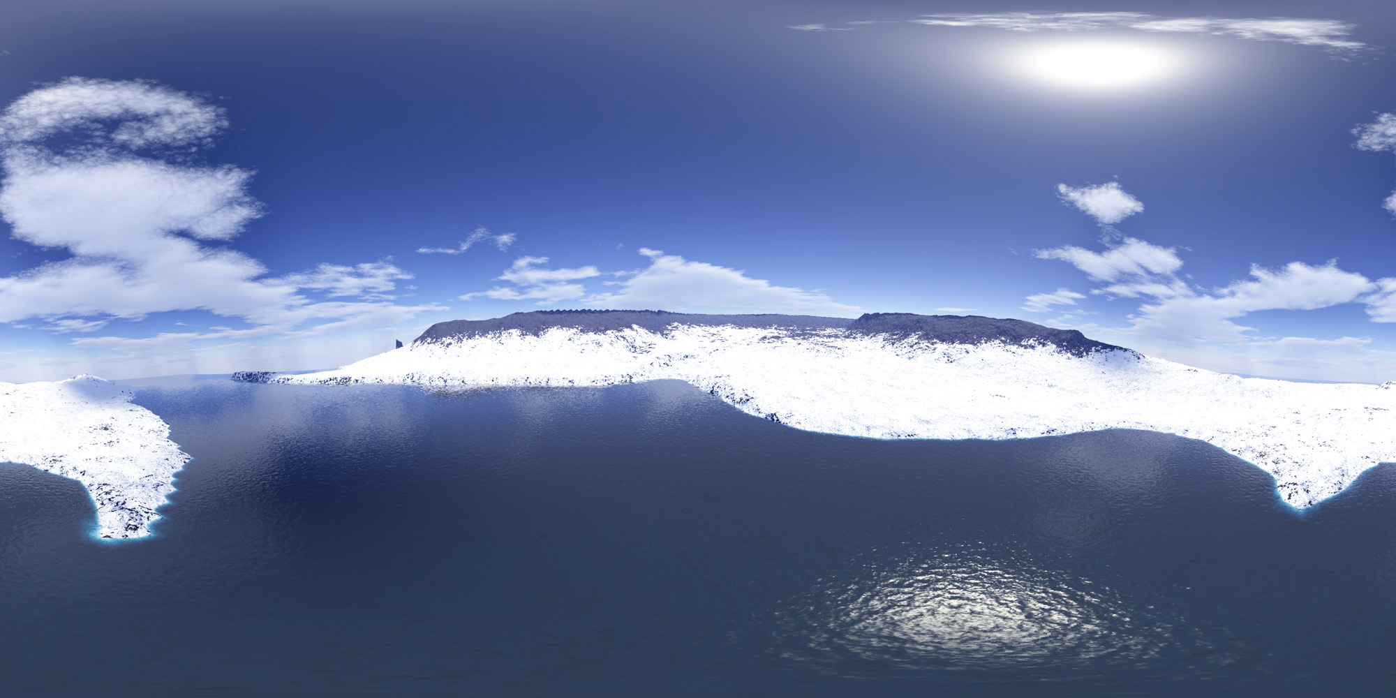
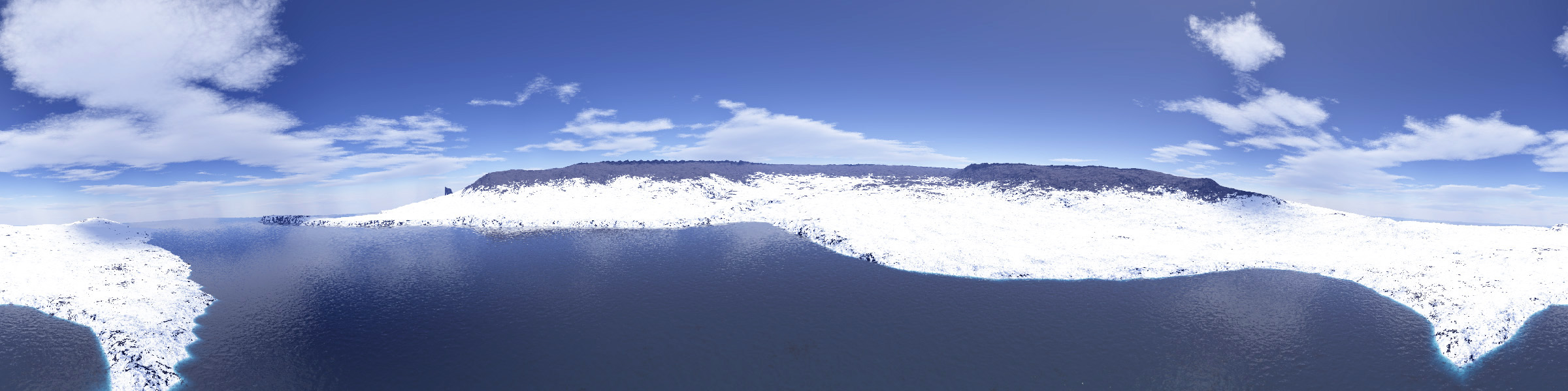
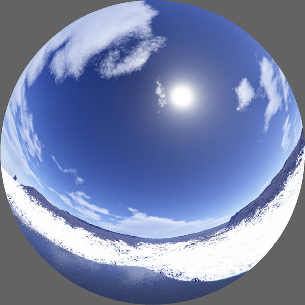
Motivation There are a number of environments in which one might want to create content using Terragen but for which Terragen doesn't provide explicit support eg: stereoscopic projection, fisheye frames for planetarium domes, panoramic images. The following describes a utility that solves this problem and as a side effect conforms to conventions that allow time consuming animation rendering to be performed locally on a large rendering cluster of 200+ processors. The utility is called "tgs_interp" mostly because it provides keyframe interpolation (supported by keyframe files in Terragen called a .tgs file). The basic work flow is to create a tgs file using Terragen or plug-ins, use tgs_interp to read this tgs file and instruct it to create a number of other tgs files which will then be read and rendered by Terragen. In the case of stereoscopic projection two tgs frames result from each interpolated frame. For cubic projection 5 or 6 tgs frames result for each interpolated frame. The utility is written for UNIX command line operation, currently compiled for Mac OS-X and Linux. Usage: tgs_interp [options] tgsfile Options -n n number of tween frames (default: 1) -c n calculate cubic views, 5 or 6 (default: off) -s n calculate stereo pairs, supply eye separation (default: off) -p n add a pitch offset in degrees, positive pitch forward (default: 0) -f n tgs splitting mode, 0=single, 1=lots, 2=stereo, 6=cubic -z n adjust camera height (default: 0)Projection options The two environments not directly supported by Terragen and addressed by this utility are:
This option determines the format of the output tgs file(s). The options are as follows.
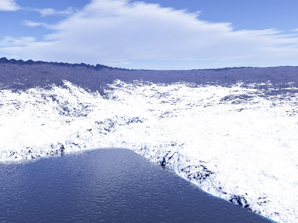
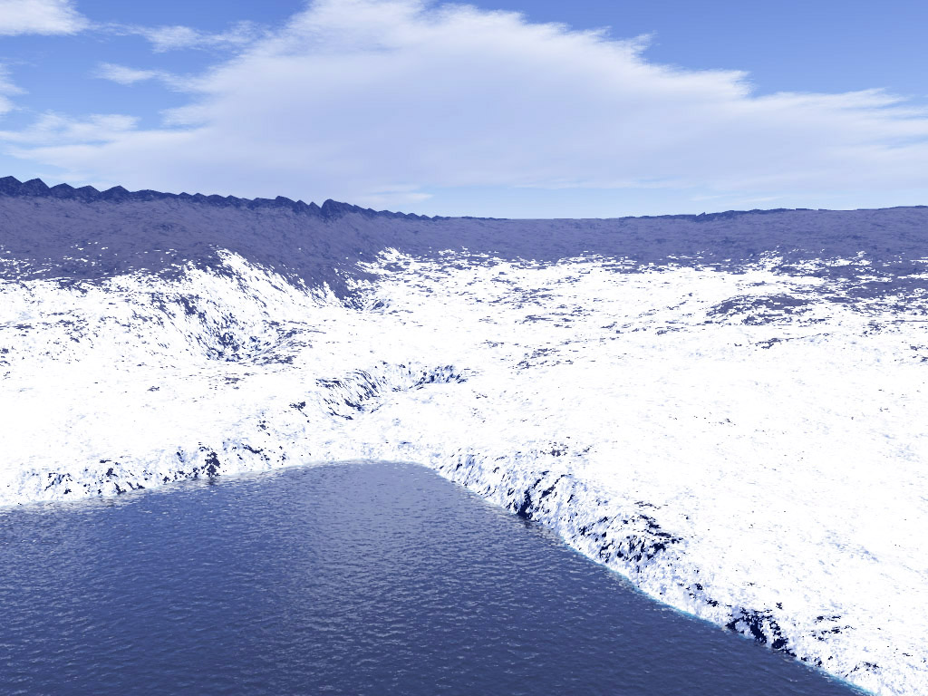
Notes on stereoscopic rendering There are a number of ways of formulating and setting up stereoscopic rendering, the approach taken here will be the correct parallel camera method and since Terragen doesn't support offaxis frustums it will be based upon the techniques described here. In essence this involves rendering frustums that are slightly wider than desired and truncating the images to give the correct stereo pairs. The following example outlines how the author would set up a stereoscopic rendering using Terragen and tgs_interp.
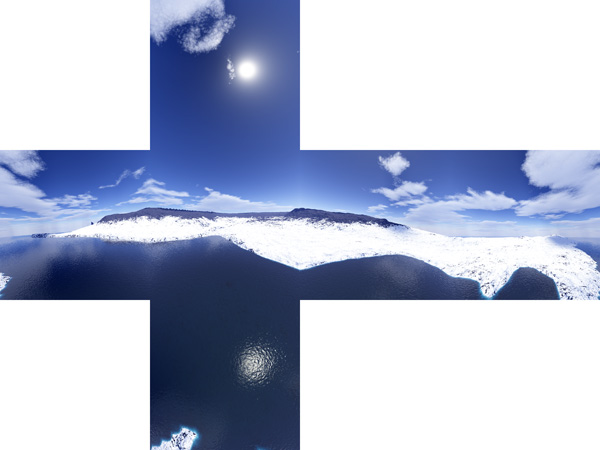
Notes on cubic rendering and derived projections The width and height of the rendered image should be set equal before rendering. The zoom factor set by the user will be reset to 1, in other words a horizontal (and vertical) aperture of 90 degrees.
Further notes
|