Various distributed rendering examplesThe following are examples of distributed rendering of either single high resolution images or animation sequences.Compiled by Paul Bourke
Spiral VaseModel and animation by Dennis MillerCopyright © 1999
Software: PovRay and MPI 
There are a number of ways one can render an animation using a standard package (such as PovRay) and exploit a collection of computers. For efficiency a prime objective is to ensure the machines are all busy during the time it takes to render the entire animation. The most straightforward way of distributing the frames is to send the first N frames to the first computer, the second N frames to the next computer and so on, where N is the total number of frames divided by the numbers of computers available. 
The problem with this approach is that most animations don't have a uniform rendering time per frame. The above example illustrates this point, the frames at the start of the animation take seconds to render while other frames take many minutes. Sending contiguous time chunks to each computer means that many of the computers will be standing idle while the animation will not be complete until those processing the more demanding pieces are finished. A much more balanced approach is to interleave the frames as illustrated below 
There are a number of ways this can be accomplished using PovRay, the method chosen here was to create an ini file containing all relevant/required settings including Initial_Clock, Final_Clock, Initial_Frame, and Final_Frame. Scripts are then created that invoke PovRay on each machine (using rsh) with the appropriate +SFn and +EFn command line arguments with the appropriate value of n. An alternative is to to develop tools using one of the parallel processing tools available, for example, MPI or PVM. Using this approach a "master" processes can additionally check the load on the available machines and only distribute the next frame given some suitably low value. This can be particularly important in a multi-user environment where simply "nicing" the rendering may not be user friendly enough, for example, the renderings may require significant resources such as memory.
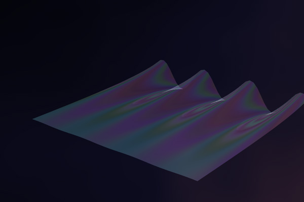
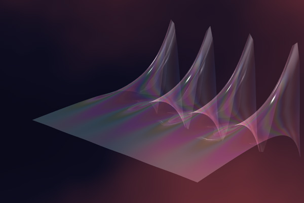
WavesModel and animation by Dennis MillerCopyright © 1999
Software: PovRay and MPI 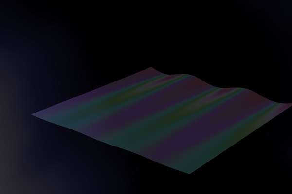
Water SunModel and animation by Dennis MillerCopyright © 2000
Software: MegaPov and MPI 
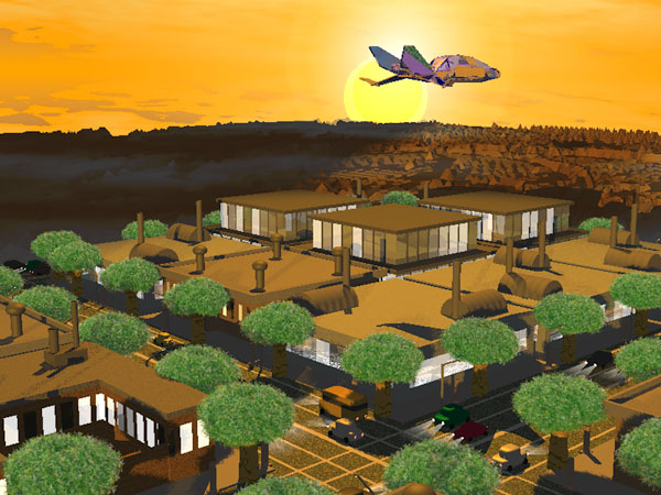
Spacecraft HangarModel and animation by Justin Watkins"Scout craft taking off from a maintenance hangar on Luna Base 4" Copyright © 1999
Software: PovRay and MPI 
Glass CloudModel and animation by Morgan LarchCopyright © 1999
Software: PovRay and MPI 
AddictModelling/rendering by Rob RichensCopyright © 2001
Concept and direction by Dale Kern.
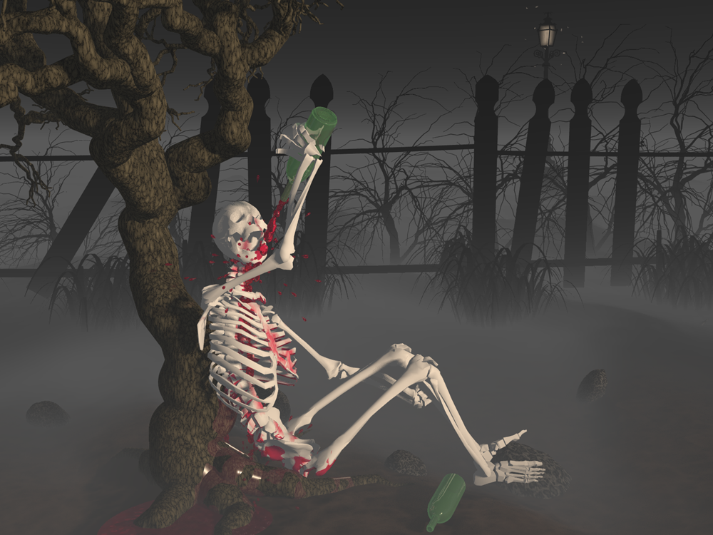
Using locally developed scripts and CPU cycles on a 32 processor PIII and 64 processor Dec Alpha farm. Astrophysics and Supercomputing, Swinburne University of Technology. November 2001
EscapeModelling/rendering by Rob RichensCopyright © 2006
Concept and direction by Dale Kern.
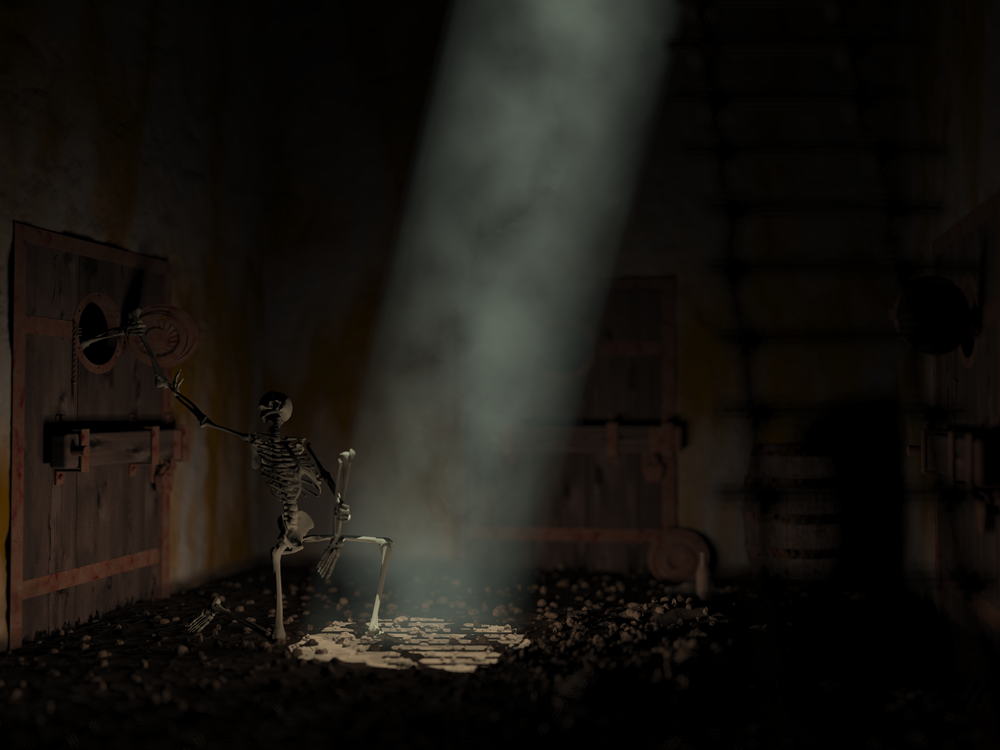
Using locally developed scripts and the PBS batch queue system. The image is rendered across a large number of processors as a series of narrow strips which are reassembled at the end. CPU cycles from a 176 CPU SGI Altix, IVEC, Western Australia. November 2006
Given a number of computers and a demanding POVRAY scene to render, there are a number of techniques to distribute the rendering among the available resources. If one is rendering an animation then obviously each computer can render a subset of the total number of frames. The frames can be sent to each computer in contiguous chunks or in an interleaved order, in either case a preview (every N'th frame) of the animation can generally be viewed as the frames are being computed. Typically an interleaved order is preferable since parts of the animation that may be more computationally demanding are split more evenly over the available computing resources. In many cases even single frames can take a significant time to render. This can occur for all sorts of reasons: complicated geometry, sophisticated lighting (eg: radiosity), high antialiasing rates, or simply a large image size. The usual way to render such scenes on a collection of computers is to split the final image up into pieces, rendering each piece on a different computer and sticking the pieces together at the end. POVRAY supports this rendering by the ini file directives
Width=n Start_Row=n End_Row=n Start_Column=n End_Column=n There are a couple of different ways an image may be split up, by row, column, or in a checker pattern.  It turns out that it is normally easier to split the image up into chunks by row, these are the easiest to paste together automatically at the end of the rendering. Unfortunately, the easiest file formats do deal with in code are TGA and PPM, in both these cases writing a "nice" utility to patch the row chunks together is frustrated by an error that POVRAY makes when writing the images for partial frames. If the whole image is 800 x 600 say and we render row 100 to 119, the PPM file should have the dimensions in its header state that the file is 800 x 20. Unfortunately it states that the image is 800 x 600 which is obviously wrong and causes most image reading programs to fail! I'd like to hear any justification there might be for this apparently trivial error by POVRAY. [A fix for this has been submitted by Jean-François Wauthy for PNG files, see pngfix.c] For example the ini file might contain the following
Width=800 Start_Row=100 End_Row=119 A crude C utility to patch together a collection of PPM files of the form filename_nnnn.ppm, is given here (combineppm.c). You can easily modify it for any file naming conventions you choose that are different from those used here. So, the basic procedure if you have N machines on which to render your scene is to create N ini files, each one rendering the appropriate row chunk. Each ini file creates one output image file, in this case, in PPM format. When all the row chunks are rendered the image files are stuck together. How you submit the ini files to the available machines will be left up the reader as it is likely to be slightly different in each environment. Two common methods are: using rsh with the povray command line prompt, or writing a simple application for parallel libraries such as MPI or PVM. The later two have the advantage that they can offer a degree of automatic error recovery if a row chunk fails to render for some reason. The following crude C code (makeset.c) illustrates how the ini files might be automatically created. Of course you can add any other options you like to the ini file. The basic arithmetic for the start and stop row chunks is given below, note that POVRAY starts its numbering from row 1 not 0!
End_Row=((i + 1) * HEIGHT) / N With regard to performance and efficiency.....if each row chunk takes about the same time to render then one gets a linear improvement with the number of processors available. (This assumes that the rendering time is much longer compared to the scene loading time). Unfortunately this is not always the case, the rows across the sky might take a trivial length of time to render while the rows that intersect the interesting part of the scene might take a lot longer. In this case the machines that rendered the fast portions will stand idle for most of the time. For example consider the following scene rendered simultaneously in equal height slices on 48 machines, there is over a factor 1000 in the rendering time for the dark row chunks compared to the lighter shaded row chunks. In this case the cause is easy to determine, any row with a tree blows out the rendering time.  One way around this is to split the scene into many more row chunks than there are computers and write a utility that submits jobs to machines as they become free. This isn't hard to do if you base your rendering around rsh and it is reasonably easy with MPI or PVM once you understand how to use those libraries.
Note 
All these techniques assume one has a scene that takes a significant time to render. The experimentation described above was performed on a scene provided by Stefan Viljoen that for fairly obvious reasons (trees) is extremely CPU demanding. If you would like to experiment yourself, the model files are provided here (overf.tar.gz). The scene, as provided, rendered with the following ini file took just over 16 hours on a farm of 48 identical DEC XP1000 workstations.
Height=900 Antialias=On Antialias_Threshold=0.3 Output_File_Name=overf.ppm Input_File_Name=overf.pov Output_File_Type=P Quality=9 Radiosity=off
Load Balancing for Distributed PovRay RenderingWritten by Paul BourkeMegaPovPlus model graciously contributed by Gena Obukhov.
Rendered using MegaPovPlus on the August 2000
The only remaining issue is how does one determine or estimate the time profile and therefore the width of each strip. The approach taken was to pre-render a small image, 64 pixels wide say, render it in one pixel wide columns timing each column. The time estimates from this preview were fitted by a Bezier curve which is then used to compute the strip width for the large rendering. A continuous fit such as a Bezier is required since the determination of the strip width is most easily done by integrating the time curve and splitting it into N equal area segments. More processes isn't always better
As a word of warning, when distributing strips to machines in a rendering farm, more machines doesn't necessarily mean faster rendering times. This can come about when there is a significant model sizes and the model files reside on one central disk. Consider a scene that takes 2 hours to render and 1 minute to load. As the number of machines (N) is increased the rendering time (assuming perfect load balancing) drops by 1/N but the model loading is limited by the disk bandwidth and when saturated the rendering machines will wait for a time proportional to N. This is a slightly surprising result and is relevant to many rendering projects where the scene descriptions (especially textures) can be large. Note that a common option is to stagger the times that the rendering machines start so they are not all reading from disk. While this certainly helps the performance of the individual nodes it doesn't improve overall rendering time. Antialiasing warning
There is a further consideration when rendering strips in PovRay, that is, antialiasing. The default antialiasing mode is "type 1" which is adaptive, non-recursive super-sampling. A quote from the manual "POV-Ray initially traces one ray per pixel. If the colour of a pixel differs from its neighbours (to the left or above) by more than a threshold value then the pixel is super-sampled by shooting a given, fixed number of additional rays." The important thing here is that this form of antialiasing isn't symmetric but depends on the left/top transition. If this is used when rendering the strips the images won't perfectly combine when joined together. This can be seen below, the scene is split into two halves, the image on the left uses type 1 and the one on the right uses type 2, note the thin band at the seam on the image on the left.
Another solution is to simply render the image at a higher resolution without any antialiasing and subsample the final image with an appropriate filter, eg: Gaussian.
|