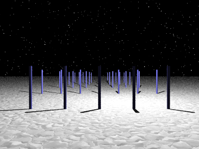
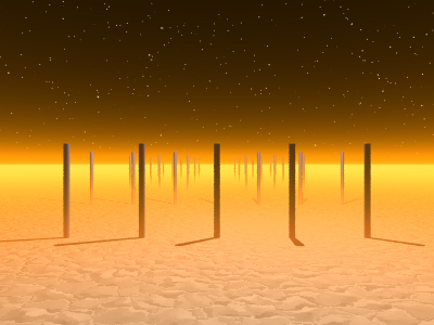
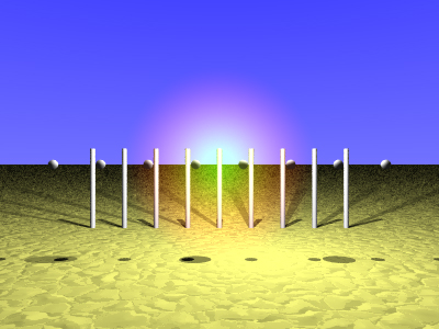
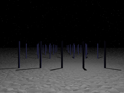
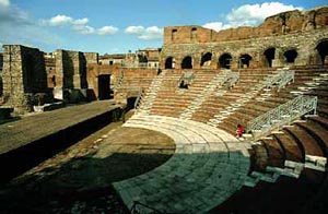
Various POVRay Related MaterialPovRay for scientific illustration: diagrams to photo-realism. POVRay density (DF3) files: Using POVRay as a volume renderer. Frustum clipping polygonal models for POVRay. CSG modelling, bump maps, media, quality settings, texture billboarding, fog, lens types, QuickTime VR navigable objects. Representing WaveFront OBJ files in POVRay.
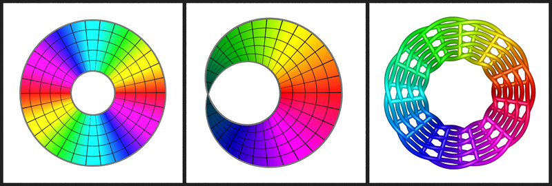
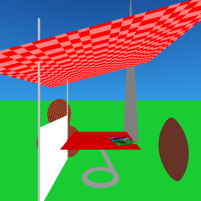
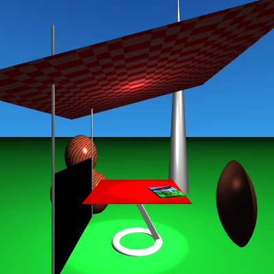
PovRay for scientific illustration: diagrams to photorealismWritten by Paul BourkeMay 2006 The following is a short illustration of how PovRay (a free and powerful rendering engine) can be used to create images suitable for all stages of scientific research: investigation, diagrams for papers, and high quality images for promotional purposes. The three versions below are all described identically with regard to their geometry, the differences are only in how that geometry is rendered. Note the PovRay files provided here are only intended to illustrate the rendering modes, there are external (#included) files and textures not included. Figure 1 - the triptych [figure1.pov]This is the diagram as it appeared in the journal, almost all features of PovRay are turned off, it is flat shaded, one light source at the camera position, no shadows, and the camera employs an orthographic projection. This is in the style typical of scientific or mathematical illustration. Figure 2 [figure2.pov] This is similar to the renderings of the geometry that were created during the scientific visualisation process. This is exactly the same geometry as in figure 1 above, the only difference is the rendering style, surface properties, lighting, and the placement of the components. Images of this form were used to solidify concepts in geometry and for discussion between researchers. 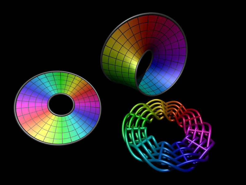
Figure 3 [figure3.pov] The following was created as a presentation form of the same geometry. It is rendered using radiosity (MegaPov), the lighting is defined by a HDR lighting environment of the staff tearoom (there are no other light sources). Additionally the result of the rendering was saved as a HDR image file (Radiance format) allowing exposure changes and filtering to be applied in post production without the usual artefacts that one encounters when using a limited 8 bits per r,g,b colour space. The page in the scene is how the diagram in figure 1 appeared in the draft version of the published paper. The final image was rendered at 6400 x 4800 pixels for a high resolution photographic print. 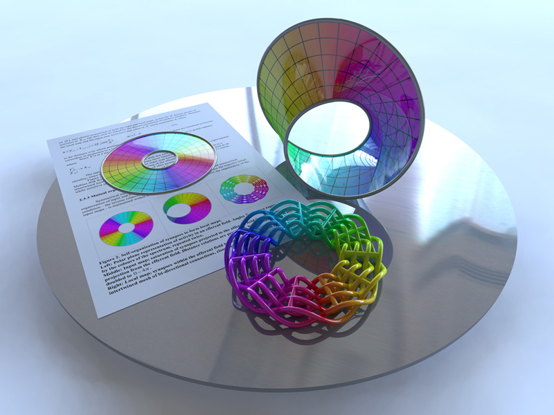
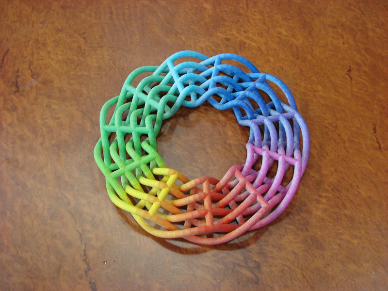
Rapid prototype model
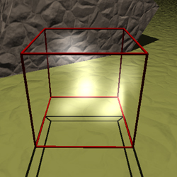
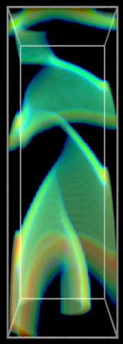
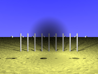
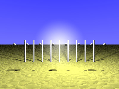
POVRay, from version 3.1, supports a volumetric density media. This can be used to represent arbitrary media distributions, the volumetric values can be mapped to variations in density (using a density_map) or colour (using a colour_map). While this was primarily introduced as a powerful way to specify user defined media effects, it can also be used for certain volume rendering applications. For a simple example, the following contains a number of Gaussian smeared points of different standard deviations. The POVRay file is here: example.pov, note that the density in this example just controls the emission in the media. While the density_map in this case is quite boring, different mappings are possible depending on the application. For more information on the media settings see the POVRay documentation.
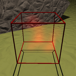
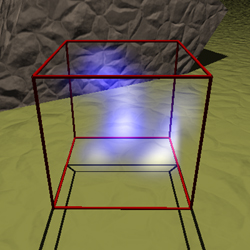
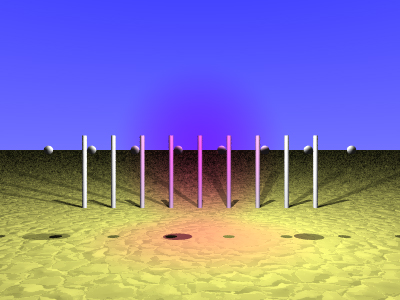
A couple of simple examples adding a colour map are given below.
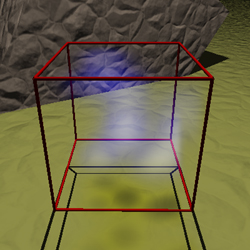
By adding an absorption "absorption <1,1,1>" and turning on media interaction for the light sources, the media will cast shadows.
The format of a DF3 file is straightforward, it consists of a 6 byte header containing the 3 dimensions of the volume, this is followed by the voxel cells. Each voxel can be represented as a single byte (unsigned char), a 2 byte integer (unsigned short), or 4 byte integer (unsigned int). The 2 and 4 byte versions are written as big-endian (Intel chips are little endian, Mac PowerPC or G4/G5 are big-endian). POVRay works out which data type is used by the size of the file. The voxels are ordered as x varying the fastest, then y, and finally z varying the slowest. The following gives the outline of how one might create a 3D volume and save it as a DF3 file where each voxel is a single unsigned byte. Using floats for the volume is simply to make the maths easier if one is creating arbitrary functions. For many applications it is OK to use short ints or even char directly. Note the endian of the short ints in the header and the order the volume voxels are written.
   int i,j,k;
   int nx=256,ny=256,nz=256;
   float v,themin=1e32,themax=-1e32
   float ***df3; /* So we can do easier maths for interesting functions */
   FILE *fptr;

   /* Malloc the df3 volume - should really check the results of malloc() */
   df3 = malloc(nx*sizeof(float **));
   for (i=0;i<nx;i++)
      df3[i] = malloc(ny*sizeof(float *));
   for (i=0;i<nx;i++)
      for (j=0;j<ny;j++)
         df3[i][j] = malloc(nz*sizeof(float));

   /* Zero the grid */
   for (i=0;i<nx;i++)
      for (j=0;j<ny;j++)
         for (k=0;k<nz;k++)
            df3[i][j][k] = 0;

   -- Create data volume data here --

   /* Calculate the bounds */
   for (i=0;i<nx;i++) {
      for (j=0;j<ny;j++) {
         for (k=0;k<nz;k++) {
            themax = MAX(themax,df3[i][j][k]);
            themin = MIN(themin,df3[i][j][k]);
         }
      }
   }
   if (themin >= themax) { /* There is no variation */
       themax = themin + 1;
       themin -= 1;
   }

   /* Write it to a file */
   if ((fptr = fopen("example.df3","w")) == NULL)
      return(FALSE);
   fputc(nx >> 8,fptr);
   fputc(nx & 0xff,fptr);
   fputc(ny >> 8,fptr);
   fputc(ny & 0xff,fptr);
   fputc(nz >> 8,fptr);
   fputc(nz & 0xff,fptr);
   for (k=0;k<nz;k++) {
      for (j=0;j<ny;j++) {
         for (i=0;i<nx;i++) {
            v = 255 * (df3[i][j][k]-themin)/(themax-themin);
            fputc((int)v,fptr);
         }
      }
   }
   fclose(fptr);
If 2 or 4 byte voxels are being saved from a little-endian machine (Intel) then the following macros may be helpful.
#define SWAP_2(x) ( (((x) & 0xff) << 8) | ((unsigned short)(x) >> 8) )
#define SWAP_4(x) ( ((x) << 24) | \
         (((x) << 8) & 0x00ff0000) | \
         (((x) >> 8) & 0x0000ff00) | \
         ((x) >> 24) )
#define FIX_SHORT(x) (*(unsigned short *)&(x) = SWAP_2(*(unsigned short *)&(x)))
#define FIX_INT(x)   (*(unsigned int *)&(x)   = SWAP_4(*(unsigned int *)&(x)))
So for example to write 2 bytes (unsigned short) then one have the writing loop as follows.
   for (k=0;k<nvol;k++) {
      for (j=0;j<nvol;j++) {
         for (i=0;i<nvol;i++) {
            v = 65535 * (df3[i][j][k]-themin)/(themax-themin);
            FIX_SHORT(v);
            fwrite(&v,2,1,fptr);
         }
      }
   }
Further examples
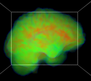
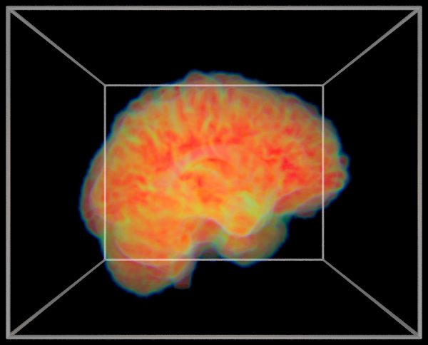
MRI "brain on fire" rendering.
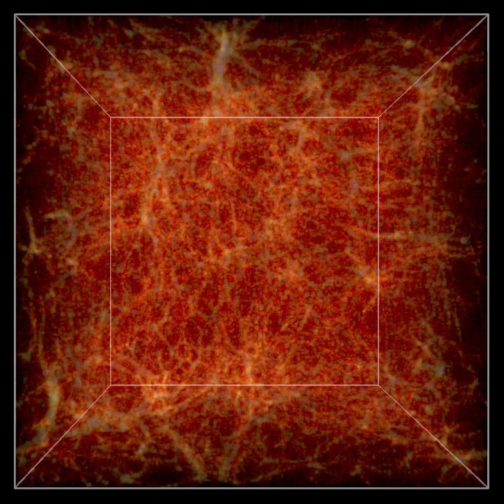
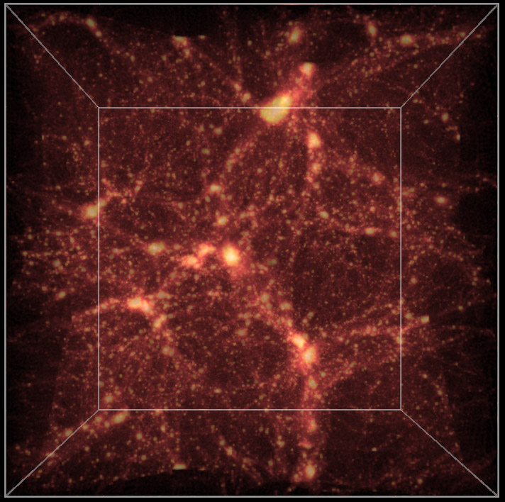
Cosmological simulations
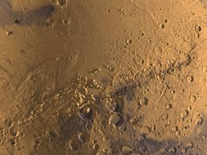
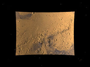
Frustum Clipping for PovRayWritten by Paul BourkeMay 2001 See also: Frustum Culling In normal rendering applications the potential exists for any piece of the geometry making up a scene to be visible or to have some effect on the visible part of the scene. For example, objects that can't be directly seen may be visible in reflective surfaces or they may cast shadows into the visible area. It is however quite common in scientific visualisation projects that there is simply too much data for PovRay to render directly. One needs to get up to "tricks", for example, creating geometry at variable resolutions depending on the distance from the camera. Another trick that will discussed here is to prune away any geometry not directly visible. The particular rendering here involved a topology model of Mars containing over 130 million polygons. The polygonal approximation was adjusted depending on the distance of the camera to the surface to give about one polygon per pixel. In order to further reduce the polygons given to PovRay the polygons outside the view frustum were removed. 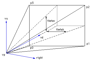 In order to compute which polygons are outside the frustum one needs to be able to define the 4 planes making up the view frustum against which each vertex of the polygons will be tested. If one defines the horizontal aperture as thetah then the vertical aperture thetav is given by the following. Where WIDTH and HEIGHT are the image dimensions. The points p0, p1, p2, p3 making up the corners of frustum can be computed using the C source below. p0 = vp; p0.x += vd.x - right.x*tan(thetah/2) - vu.x*tan(thetav/2); p0.y += vd.y - right.y*tan(thetah/2) - vu.y*tan(thetav/2); p0.z += vd.z - right.z*tan(thetah/2) - vu.z*tan(thetav/2); p1 = vp; p1.x += vd.x + right.x*tan(thetah/2) - vu.x*tan(thetav/2); p1.y += vd.y + right.y*tan(thetah/2) - vu.y*tan(thetav/2); p1.z += vd.z + right.z*tan(thetah/2) - vu.z*tan(thetav/2); p2 = vp; p2.x += vd.x + right.x*tan(thetah/2) + vu.x*tan(thetav/2); p2.y += vd.y + right.y*tan(thetah/2) + vu.y*tan(thetav/2); p2.z += vd.z + right.z*tan(thetah/2) + vu.z*tan(thetav/2); p3 = vp; p3.x += vd.x - right.x*tan(thetah/2) + vu.x*tan(thetav/2); p3.y += vd.y - right.y*tan(thetah/2) + vu.y*tan(thetav/2); p3.z += vd.z - right.z*tan(thetah/2) + vu.z*tan(thetav/2); Where vp is the view position vector, vd is the unit view direction vector, vu is the unit up vector, and right is the unit vector to the right (the cross product between vd and vu). The 4 frustum planes are (vp,p0,p1), (vp,p1,p2), (vp,p2,p3), (vp,p3,p0) from which the normal of each plane can be computed. A simple C function that determines which side of a plane a vertex lies might be as follows.
/*
   Determine which side of a plane the point p lies.
   The plane is defined by a normal n and point on the plane vp.
   Return 1 if the point is on the same side as the normal,
   otherwise -1.
*/
int WhichSide(XYZ p,XYZ n,XYZ vp)
{
   double D,s;

   D = -(n.x*vp.x + n.y*vp.y + n.z*vp.z);
   s = n.x*p.x + n.y*p.y + n.z*p.z + D;

   return(s<=0 ? -1 : 1);
}
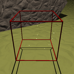
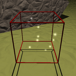
The example below shows a portion of the landscape rendered on the left. Moving the camera back a bit shows that the geometry (of the whole planet) has been clipped to remove any polygons not within the view frustum. Note that as well as frustum clipping, back facing polygons have also been removed.
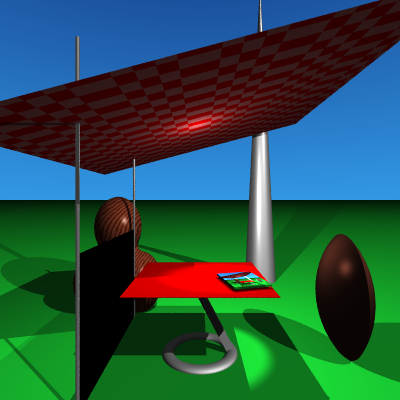
POVRAY CSG modellingWritten by Paul BourkeFebruary 1998 The following image and accompanying geometry file csg.pov illustrate the basics of the CSG (Constructive Solid Geometry) operations supported by POVRAY. The operations are performed on an intersecting circle and cylinder. Note that while the union and merge appear to give the same result, in the later the interior structure does not exist. This can be demonstrated by doing the rendering using a transparent material. 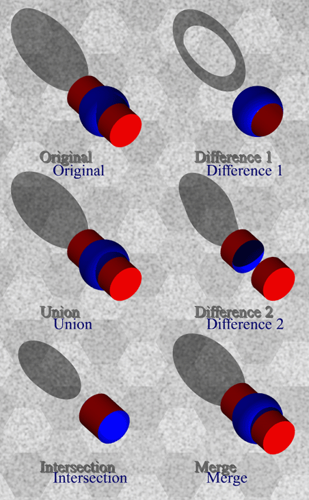
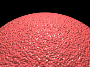
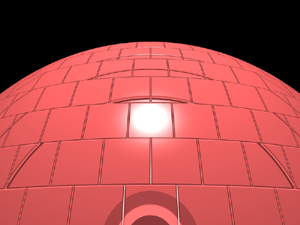
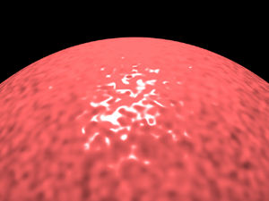
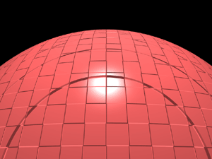
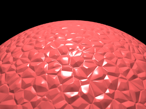
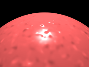
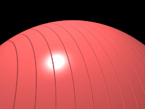
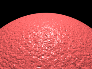
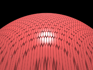
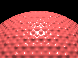
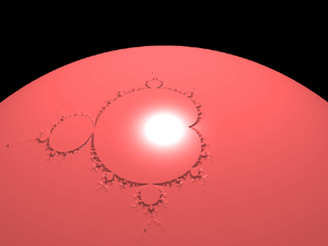
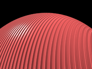
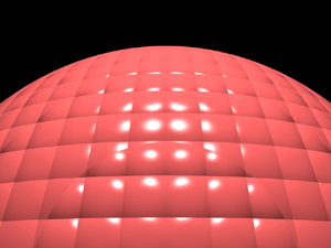
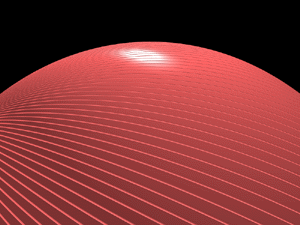
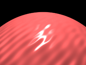
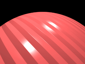
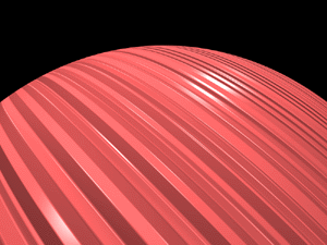
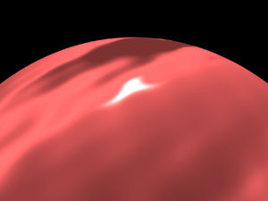
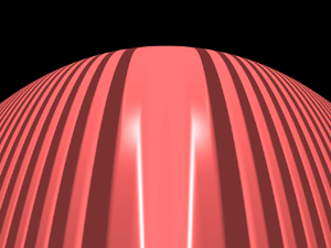
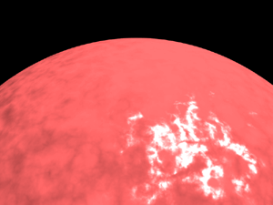
Bump Maps in PovRayWritten by Paul BourkeApril 2001
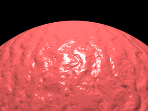
Bump maps are a way of creating the appearance of surface detail
without needing to create additional geometric detail. This is achieved by
perturbing the normals at each point on the surface. Since the
normal is used to determine how light interacts with the surface
the appearance of the surface is affected. The effect is very
powerful, in some of the examples below it is hard to imagine
that the surface hasn't been geometrically modified.
Media (PovRay 3.5)Written by Paul BourkeAugust 2002
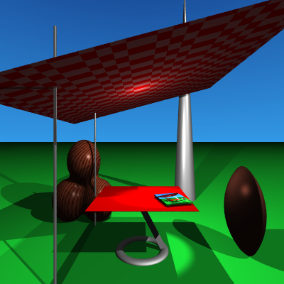
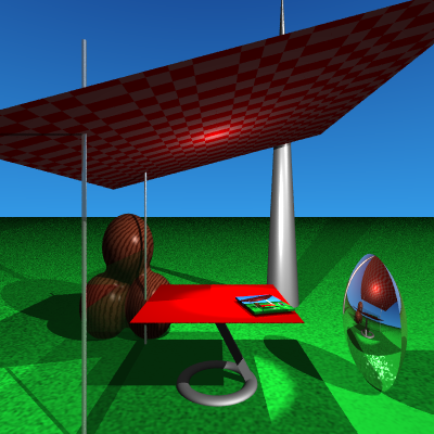
POVRAY quality settingsWritten by Paul BourkeJune 1999, updated for version 3.6 Oct 2006 The following illustrates renderings from POVRAY using the different quality settings. The scene being rendered for this example is quality.pov. The quality setting in POVRAY is set by using +Qn on the command line or Quality=n in a ".ini" file. All the rendering below were done with antialiasing on (otherwise default antialiasing settings) and rendered at 400x400, the relative times are multiples of the quality=1 raytracing time.
Texture billboarding in PovRayWritten by Paul BourkeMay 2002 Billboarding is a well established technique that maps a texture onto a planar surface that stays perpendicular to the camera. It is commonly used in interactive OpenGL style applications where textures are a much more efficient means of representing detail than creating actual geometry. The classic example is to represent pine trees (relatively radially symmetric), the texture image of the tree always faces the camera giving the impression of a 3D form. The example that will be used here is the creation of a galaxy that rotates slowly and stays facing a camera that moves along a flight path. For each section and image below a PovRay file is provided which illustrates the step and can be used to create the image. path. PovRay default texture coordinates (default.pov)The texture will be mapped onto a disc, used because the galaxy images were mostly circular, a polygon could just as easily have been used. The default PovRay texture lies on the x-y plane at z=0 as shown below. 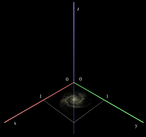 Changing the orientation (orientate.pov) The first step is to consider how to transform the texture so that it faces the camera. The camera model used here is as follows, where normally the camera position (VP), camera view direction (VD), and up vector (VU) are set by the flight path description.
camera {
   location VP
   up y
   right -4*x/3
   angle 60
   sky VU
   look_at VP + VD
}
The view direction, up vector, and right vector need to be kept mutually perpendicular, to be more precise, orthonormal. The PovRay transform statement is used to orientate the texture coordinate system so it is perpendicular to the camera view direction. 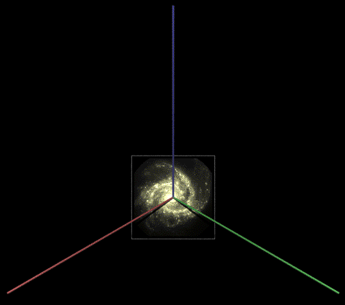 Changing the position (position.pov) In the above the disc and texture are still centered on the origin so they now need to be translated to the correct position. This could be done in the transform above (see last row of zeros) but a separate translate has been used here. 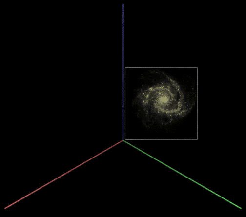 Changing the orientation (final.pov) Finally, the rotation is done, one only has the ensure that it's done at the right stage, namely while the galaxy was still centered at the origin. 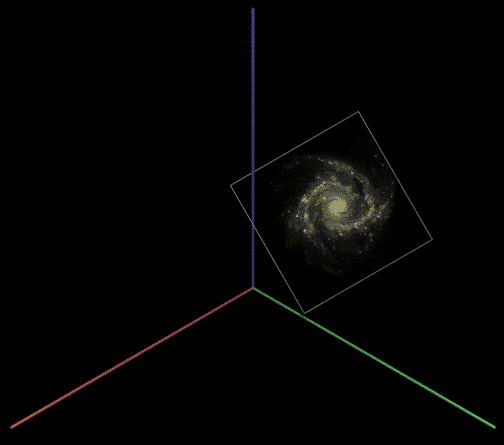
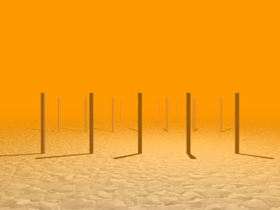
Fog (PovRay 3.5)Written by Paul BourkeAugust 2002
Making QuickTime Navigable objects using PovRayWritten by Paul BourkeApril 2000 QuickTime VR navigable objects are one of the original features (along with panoramic) Apple built into QuickTime after simple movie playing. They allow exploration of an object by moving a virtual camera around the object, generally on the surface of a sphere. Internally they are just a linear QuickTime movie but with some extra information to indicate which frame sets form the lines of longitude and latitude. The three steps in creating a QT navigable object are as follows:
The rest of this document will describe how to perform the first step above using PovRays animation support based upon the clock variable, namely, creating all the images required and in the correct order. In polar coordinates (R,Theta,Phi), sometimes called spherical coordinates, given a fixed radius (R) all the points lie on a sphere. The two angles (Theta,Phi) determine the lines of longitude (0 to 360) and latitude (90 to -90) respectively. 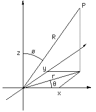
These lines of latitude and longitude can be "unwrapped" from the sphere and represented as a grid. 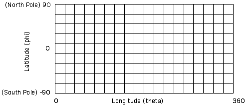
QuickTime VR object movies allow any rectangular part of this grid to be used. In most cases the entire grid is used in which case panning right past theta=360 will wrap to theta=0 for any line of latitude. Note that the line along the top and bottom edge of the grid map to a single point at the north and south pole. Whichever part of the grid is used one will need to give the longitude and latitude bounds to the software that performs step 3 above. In the following example using PovRay the object to be explored is assumed to be located at the origin, if this isn't the case it can readily be translated there or the PovRay code below modified to create the views about some other position. In the first section given below, the parameters that determine the grid resolution and range are specified. In the example here the resulting navigation will be in 5 degree steps left/right (longitude) and 10 degree steps up/down (latitude). /*
The ini file should have NLONGITUDE * (NLATITUDE + 1) frames
And a clock variable that goes across the same range
for example for NLONGITUDE = 72 and NLATITUDE = 18
Initial_Frame = 0
Final_Frame = 1367
Initial_Clock = 0
Final_Clock = 1367
Fill in the next 7 parameters
*/
#declare NLONGITUDE = 72;
#declare NLATITUDE = 18;
#declare LONGITUDEMIN = 0;
#declare LONGITUDEMAX = 360;
#declare LATITUDEMIN = -90;
#declare LATITUDEMAX = 90;
#declare CAMERARADIUS = 100;
Next we compute the polar coordinates (theta,phi) with a constant camera range given by CAMERARADIUS above. From these the camera position (VP), view direction (VD), and up vector (VU) are derived. /* Calculate polar coordinates theta and phi */
#declare DLONGITUDE = LONGITUDEMAX - LONGITUDEMIN;
#declare DLATITUDE = LATITUDEMAX - LATITUDEMIN;
#declare THETA = LONGITUDEMIN + DLONGITUDE * mod(int(clock),NLONGITUDE) / NLONGITUDE;
#declare THETA = radians(THETA);
#declare PHI = LATITUDEMAX - DLATITUDE * int(clock/NLONGITUDE) / NLATITUDE;
#if (PHI > 89.999)
#declare PHI = 89.999;
#end
#if (PHI < -89.99)
#declare PHI = -89.999;
#end
#declare PHI = radians(PHI);
#debug concat("\n****** Clock: ",str(clock,5,1),"\n")
#debug concat(" Theta: ",str(degrees(THETA),5,1),"\n")
#debug concat(" Phi: ",str(degrees(PHI),5,1),"\n")
/* Calculate the camera position */
#declare VP = CAMERARADIUS * <cos(PHI) * cos(THETA),cos(PHI) * sin(THETA),sin(PHI)>;
#declare VD = -VP;
#declare VU = <0,0,1>;
#declare RIGHT = vcross(VD,VU);
#declare VU = vnormalize(vcross(RIGHT,VD));
In the above the tweaking of PHI at 90 and -90 (the poles) is a nasty solution to the problem of creating the correct up vector (VU) at the poles, there are more elegant ways but this seems to work OK. This method works in combination with the cross product to calculate a right vector and then the correct up vector that is at right angles to the view direction. These camera variables (position, view direction and up vector) are finally combined into a camera definition which may look something like the following. camera {
location VP
up y
right x
angle 60
sky VU
look_at <0,0,0>
}
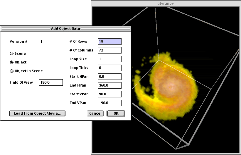
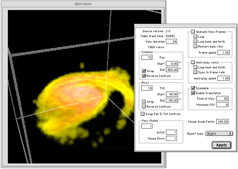
An unfortunate reality of these navigable object movies is their size. For D1 degree steps in longitude and D2 latitude, the total number of frames for a full sphere is given by ((180+D2)/D2)*(360/D1). So for the example above D1 = 5 and D2 = 10 degrees so there are 1368 frames. For a smoother sequence where there 2 degree steps in both directions there would be 16380 frames! For this reason I haven't included an actual QuickTime VR object example movie. Screen shot examples of various QT VR tools
Representing WaveFront OBJ files in POVRayWritten by Paul BourkeOctober 2012 With the introduction of the mesh2 primitive in POVRay there is now a nice one to one mapping between textured mesh files in WaveFront OBJ format and POVRay. A textured mesh in OBJ format may be represented as follows, note that long lists of vertices, normals, etc have been left out in the interests of clarity. There are essentially 4 common sections, "v" are vertices, "vn" are normals, usually one per vertex, "vt" texture uv coordinates on the range 0 to 1, and finally faces defined by indices into the vertex, normal, and texture lists.
# a comment
mtllib some.mtl
v -27.369801 -16.050600 18.092199
v -27.171200 -14.097800 17.699499
     - cut -
vn -2.350275 -1.812223 -1.067749
vn -5.281989 0.596537 -2.515623
     - cut -
vt 0.000000 0.000000
vt 0.780020 0.805009
     - cut -
usemtl materialname
f 2766/2/2766 2767/3/2767 2768/4/2768
f 2778/14/2778 2779/15/2779 2777/13/2777
     - cut -
The mapping to a POVRay mesh2 object is as follows
// a comment
mesh2 {
 vertex_vectors { 83954,
  <-27.369801,-16.050600,18.092199>,
  <-27.171200,-14.097800,17.699499>,
     - cut -
 }
 normal_vectors { 83954,
  <-2.350275,-1.812223,-1.067749>,
  <-5.281989,0.596537,-2.515623>,
     - cut -
 }
 uv_vectors { 86669,
  <0.000000,0.000000>,
  <0.780020,0.805009>,
     - cut -
 }
 face_indices { 54515,
  <2765,2766,2767>,
  <2777,2778,2776>,
     - cut -
 }
 normal_indices { 54515,
  <2765,2766,2767>,
  <2777,2778,2776>,
     - cut -
 }
 uv_indices { 54515,
  <1,2,3>,
  <13,15,13>,
     - cut -
 }
 uv_mapping
 texture { texturename }
}
Note
|
