Geometry of sports ballsWritten by Paul BourkeJanuary 2017
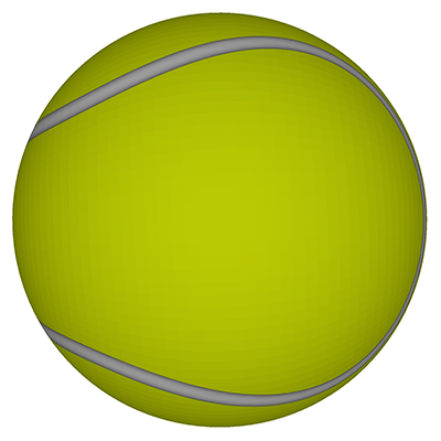
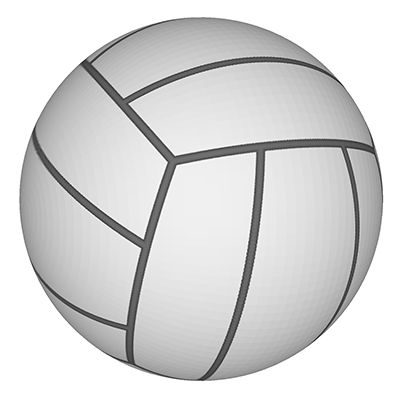
In what follows various mathematical and graphical models will be presented for the surface features of some popular sports balls. In each case the equirectangular texture will be provided along with a couple of rendered images. The intent here is not to present high quality and realistic renderings, but rather to capture the underlying geometric essence. It should be noted that in many cases there is not one design for the balls, there is variation over the years as manufacturing has evolved but also variations due to different manufactures, in some case variations arising due to patents. Tennis ball (Softball, Baseball, Basketball, Tee ball, Hurling)
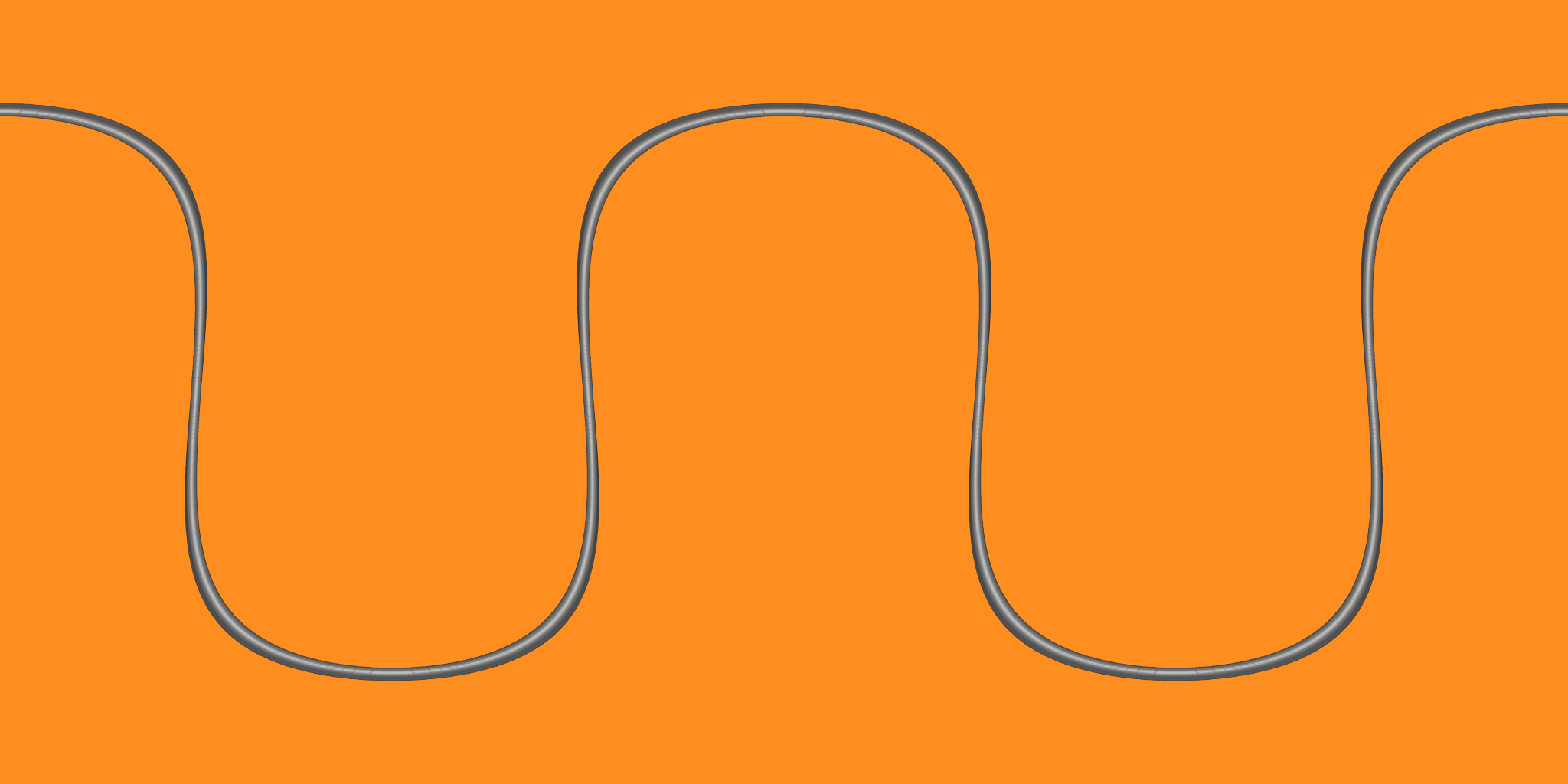
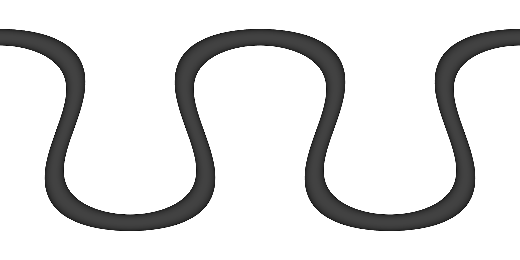
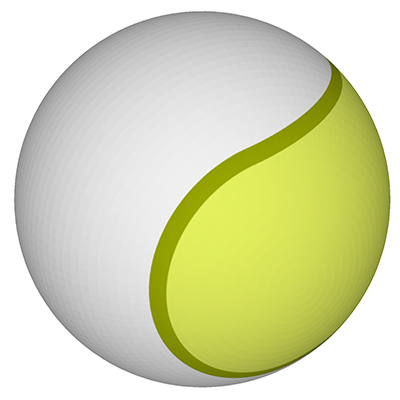
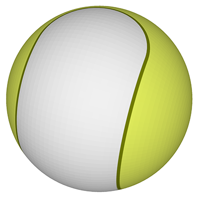
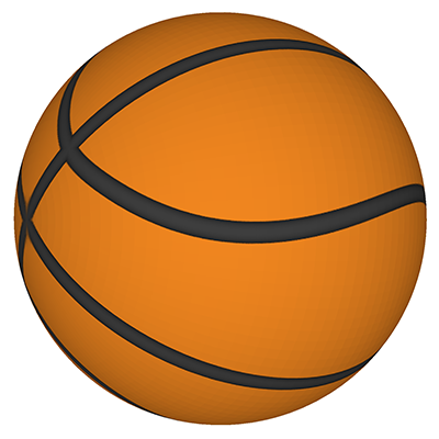
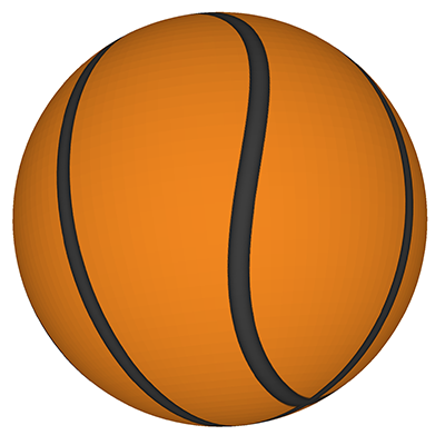
The shape of the seam on a tennis ball, like some other ball seams, arises from the initial goal of producing one 2D shape that can be cut out of a sheet of material and then stitched together in pairs. This is an example of dform surfaces. One proposed equation for the the seam is the following parametric equation y = sin(pi/2 - (pi/2 - A) cos(T)) sin(T/2 + A sin(2T)) z = cos(pi/2 - (pi/2 - A) cos(T)) Where T ranges from 0 to 4pi and parameter A in the following is 0.44.

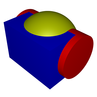
Another construction involves constructive solid geometry, namely the subtraction of a cylinder and box from a sphere.
Equirectangular projection of one half of ball, the other half is the same form rotated 180 degrees about the vertical axis and then 90 degrees along the gap axis. 
The relative size of the lobes is controlled by the relative size of the subtracted cylinder and box.
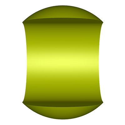
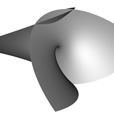
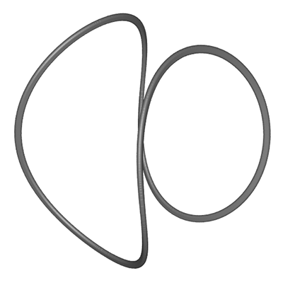
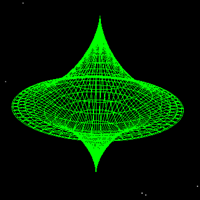
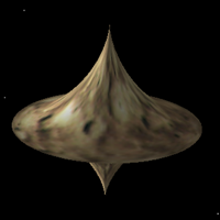
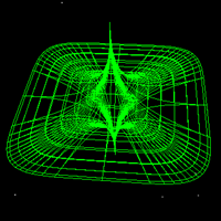
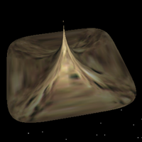
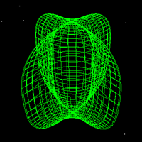
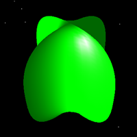
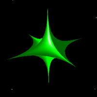
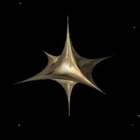
Another formation with good control over the seam spacing is to take the intersection of
an Ennepers minimal
surface with a sphere, the radius of the sphere controlling how close the
lobes are. y = v - v3 / 3 + v u2 z = u2 - v2 Where, in the figure below, -2 <= u <= 2, -2 <= v <= 2
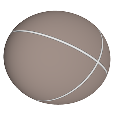
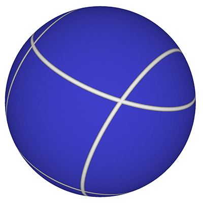
The main curved seam on a basketball can be created using the same techniques as for the tennis ball, it has an additional two seams at 90 degrees to each other. 
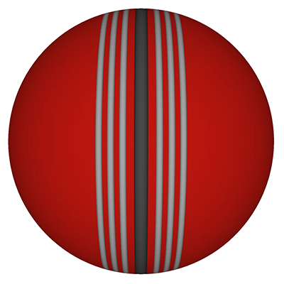
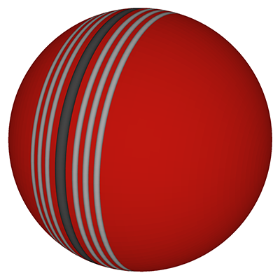
This is a rather dull case since a cricket ball only has a single seam between two hemispheres, dark line in the equirectangular below. The other curves represent the stitching which runs along lines of latitude on either side of the seam. 
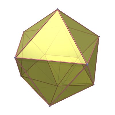
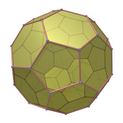
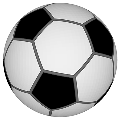
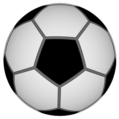
A soccer ball seam is the projection of a truncated icosahedron (see item 22 and 25) onto the surface of a sphere. There are 60 vertices, 90 seam edges, 20 regular hexagonal faces and 12 regular pentagonal faces. The truncated icosahedron is constructed by starting with an icosahedron with the 12 vertices truncated 1/3 of the distance. This creates 12 additional pentagon faces, and turns the original 20 triangular faces into regular hexagons.
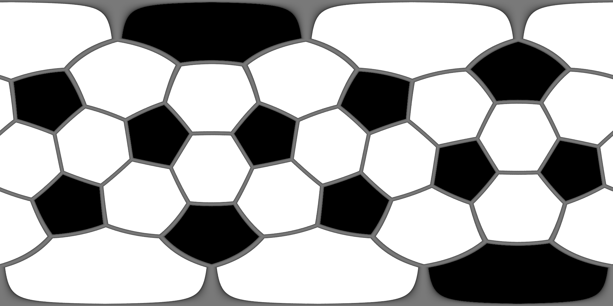
The map can be rotated to place the two hexagons at the poles making the equirectangular projection easier to understand. 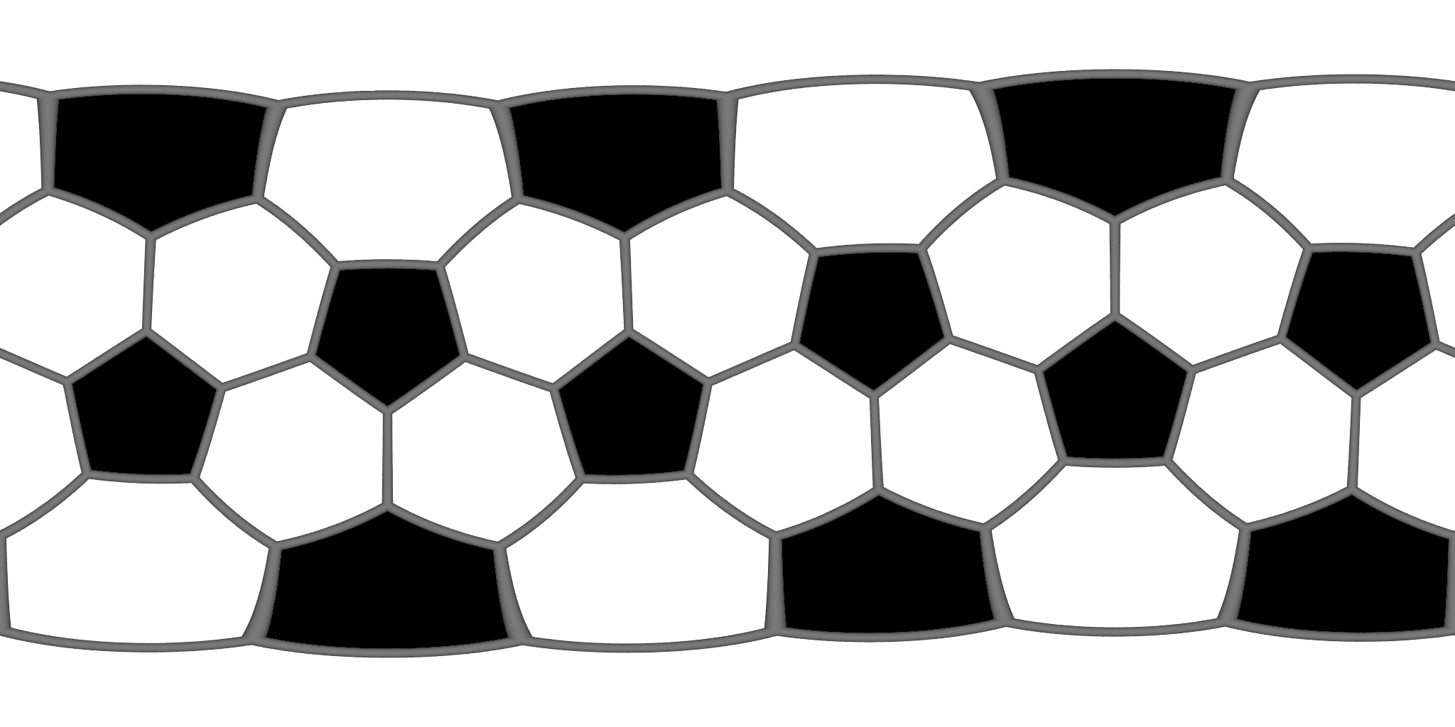
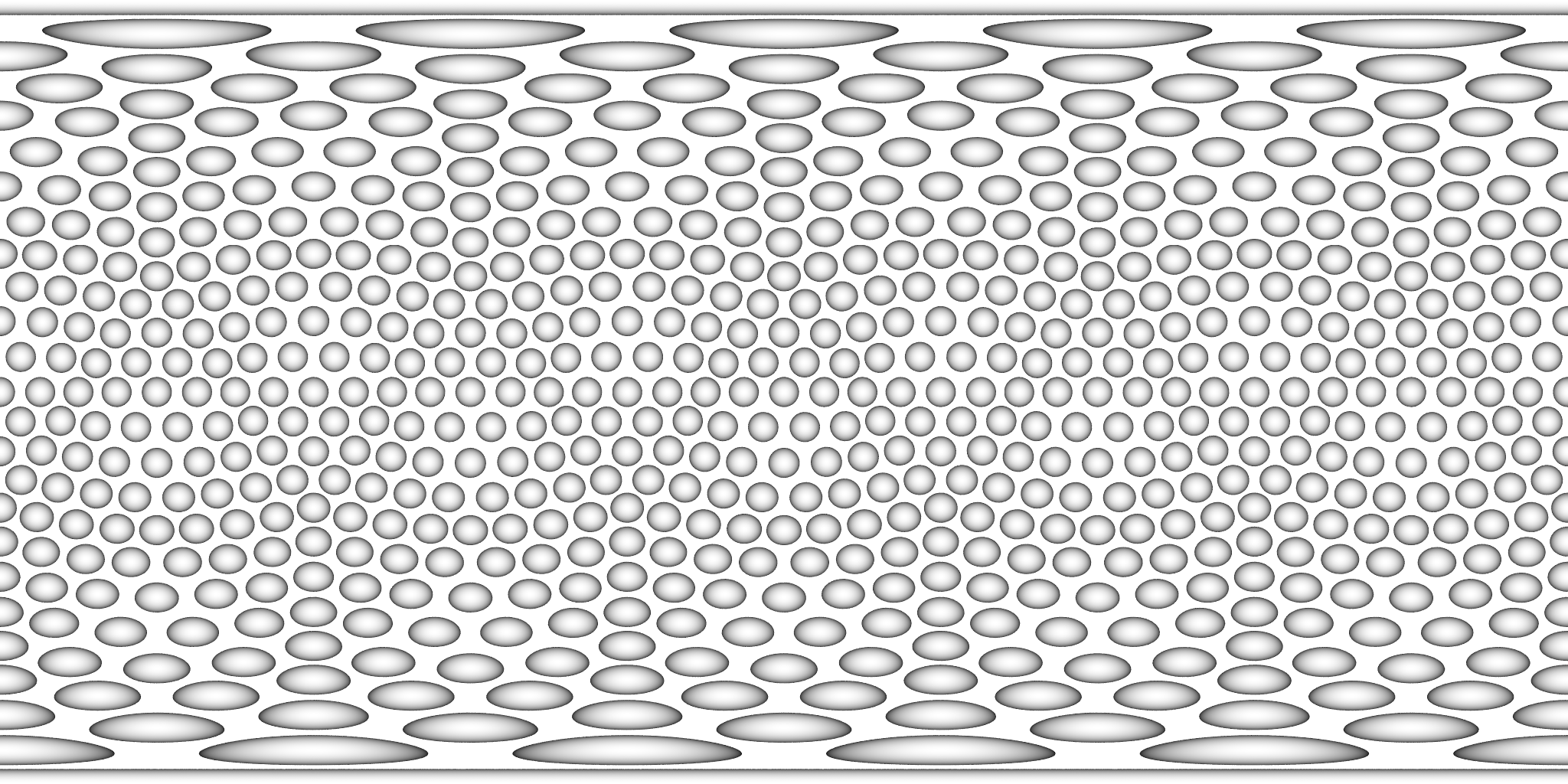
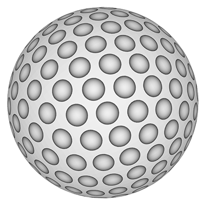
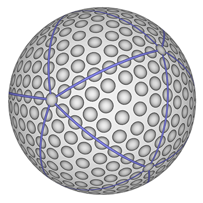
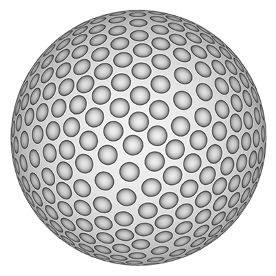
The roughness of a golf ball, introduced in the late 1800's, made for a more consistent flight path than smooth surfaces. The dimples, introduced in the early 1900's, create a turbulent layer around the ball creating a low pressure leading edge and thus less drag allowing the ball to travel further. There were disputes in the 1980's around symmetric vs non-symmetric dimple patterns, the later provided for a sort of self correction of ball spin during flight. While there are asymmetric balls they are only allowed in non-tournament games. Most balls have between 300 and 500 dimples. The example below has 308 dimples. It is formed by progressively sampling lines of latitude in equal steps with ever increasing steps in longitude and phase offsets per latitude. 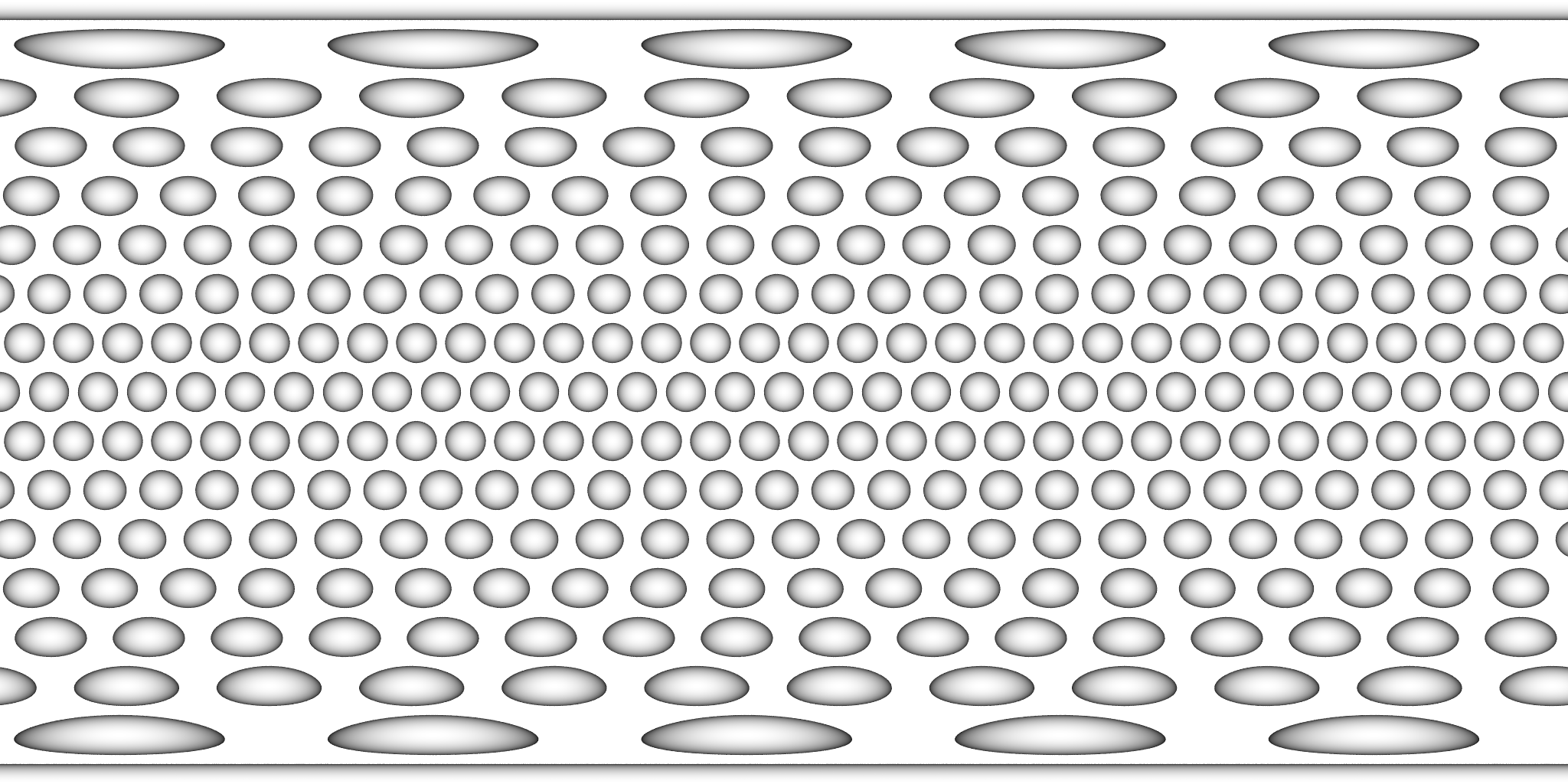
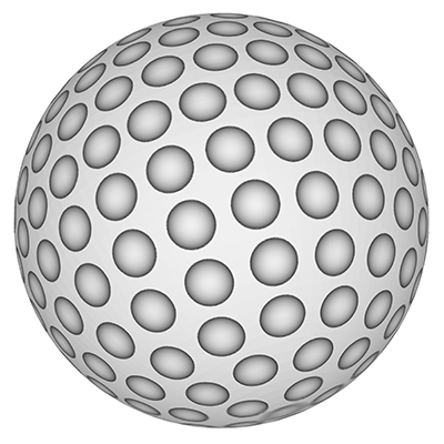
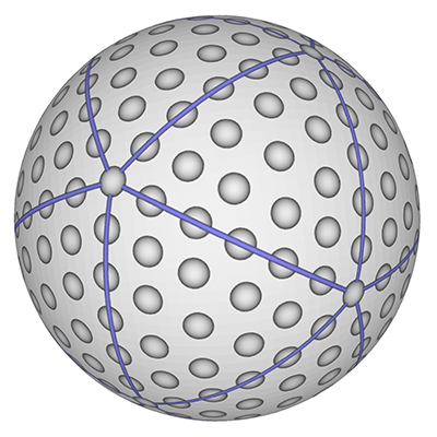
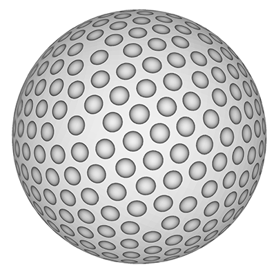
But this doesn't give the local hexagonal neighbourhood around each dimple, see the example on the right above. A more regular dimple pattern can be achieved by starting with an icosahedron and tiling each triangular face with a regular triangular array of dimples. 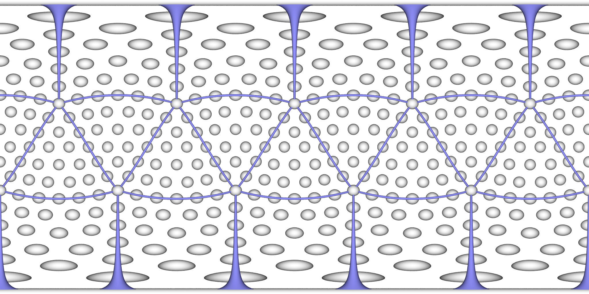
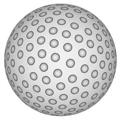
The next approach is to perform a minimisation process to distribute points on a sphere. This may be an arbitrary simulation or a spring system as described here. The following example has 500 dimples and unlike the previous methods where only certain densities can be supported, this approach can be applied to any number of dimples. 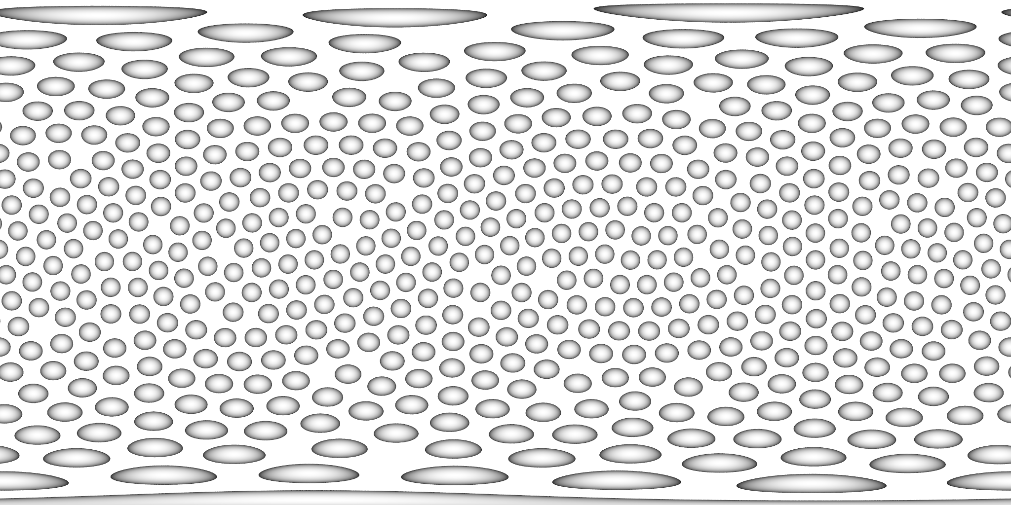
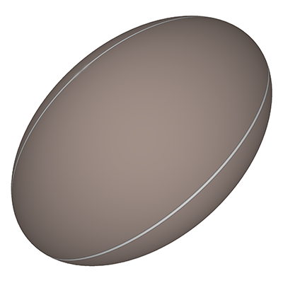
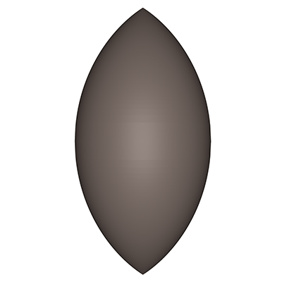
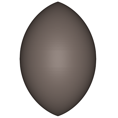
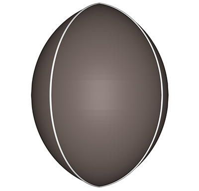
While the early rugby balls were shaped more like the American footballs, the current rugby ball is a prolate spheroid with a major to minor axis ratio of about 1.5. Besides a sphere stretched along one axis there are many other ways of describing this shape, one example being a super-ellipsoid. 
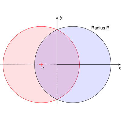
The ball shape can be represented as the intersection of two off-center circles,
rotated about the mirror axis. The design is intended to reduce drag when thrown
with a rotation along the long axis. and (x - r)2 + y2 = R2
where the range for x is 0 to R-r and the range for y is -sqrt(R2 - r2) to sqrt(R2 - r2).
The seams are the same as for the rugby football, namely, 4 lines of longitude spaced every 90 degrees about the long axis of the ball. As with most ball seams they arise from the desire to create the ball skin from a number of equal shaped and sized pieces.
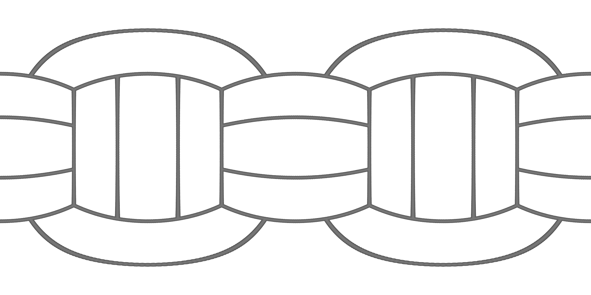
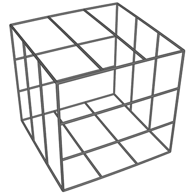
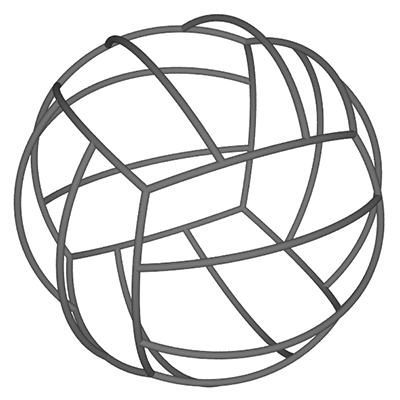
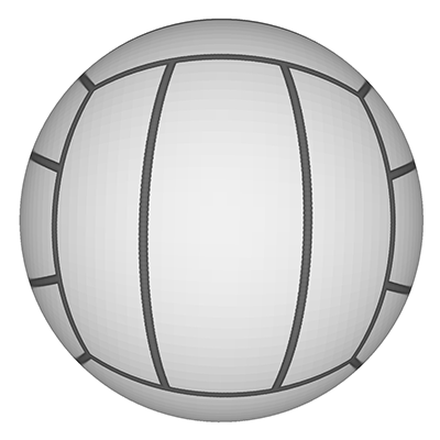
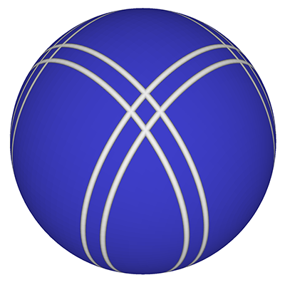
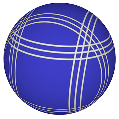
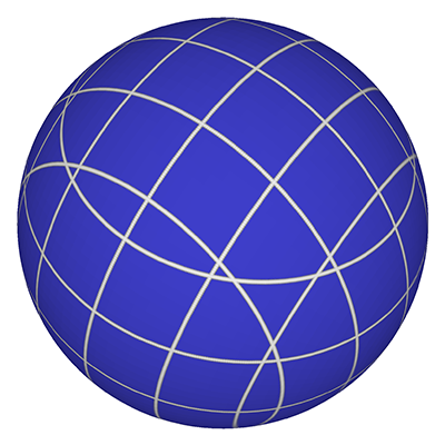
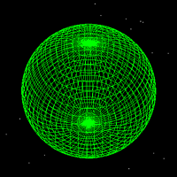
There are a few variation of the design of volley balls, the simplest to describe geometrically is presented below. One takes a cube and splits each face into three sections. The axis of the sections is the same for opposing faces of the cube, but along a different axis for each pair of opposing faces. These lines are then projected onto the surface of a sphere.
There are a wide range of designs but they are generally symmetric slices by a number of planes through a sphere, repeated on two or three axes.

There are a number of other sports balls not included here, largely because they are not interesting. Squash balls are simple spheres with only one or two small dots to indicate hardness (bounce). Similarly, ten pin bowling balls only have three finger grip holes. Pool, snooker and billiards balls may include dots (billiards) or numbers and simple bands of colour. Ping pong balls have no markings at all. Same for croquet balls, racket-ball, and polo (horseback). Prolate-spheroid and CymbelloidWritten by Paul BourkeSeptember 2002
The points on an ellipsoid (3 dimensions) satisfy the equation
Or in polar coordinates
The special case where a = b is called a prolate-spheroid, it is a sphere
with a stretch (scale factor > 1, not compression, c > a)
along one axis. The equation can be written as Where a is the equatorial radius and c the polar radius.
The example below illustrates a prolatespheroid where c = 1.5 a 
The degree of stretching is often called the eccentricity in 2 dimensions
or the ellipticity in 3 dimensions, it is defined by e is 0 for a sphere (a = c), and e approaches 1 as the prolate-spheroid become increasingly elongated.
The surface area is
The volume is
Super-ellipse and Super-ellipsoidA Geometric Primitive for Computer Aided DesignWritten by Paul BourkeJanuary 1990 See also Super-toroid, Radiance examples. This is a description of a proposed primitive for computer aided design. In 2 dimensions it includes the circle and ellipse, in 3 dimensions it has the sphere and ellipsoid as special cases. By varying its parameters it can form a continuum of other shapes. 2 dimensions - super-ellipse In 2 dimensions the super-ellipse centered at the origin is defined in parametric form as  The curve intersects the x axis at rx and -rx, it intersects the y axis at ry and -ry, ie: the super-ellipse is enclosed in a rectangle of width 2rx and height 2ry. This is the form most easily employed to draw a super-ellipse, the angle ø is varied from 0 to 2pi in suitably small steps, a line is drawn to each subsequent value of ø. 
Forming the curve using the parametric form above and uniformly varying the
angle automatically samples the curve with curvature dependent sampling. That
is, there are more samples where the curve is changing rapidly, a desirable
characteristic.
then The above can be used to form the super-ellipse (although it must be done in quadrants). Solving for y gives Varying n controls the form of the super-ellipse, some special cases are outlined below  Pictorially  Note that the super-ellipse always passes through the same points at ø = 0, pi/2, pi, 3pi/2 and so it is possible to have different values of n in each quadrant. 3 dimensions - super-ellipsoid The super-ellipse is name given to a family of shapes formed from the spherical product of two superquadratric curves. These shapes can be used to model a wide range of shapes including spheres, cylinders, and parallelepipeds as well as shapes in between. In 3 dimensions the super-ellipse centered at the origin is defined as follows
 As for the two dimensional case rx, ry, and rz are the scale factors for each axis (axis intercept). The total shape lies at the centre of a box of dimension 2rx, 2ry, 2rz. The power n1 acts as the "squareness" parameter in the z axis and n2 the squareness in the x-y plane. Some special cases of parameter n1 and n2  The super-ellipse can also be written as
where the same relationships as for the 2D case (super-ellipse) can be made,
namely Closed expressions can be derived for the normal at any point on the super-ellipsoid making many rendering calculations with lighting models easier. The normal is given by  Interestingly, if n1 and n2 are less than 2 then the equation of the normal of the super-ellipsoid is another super-ellipsoid (its dual) with n1 -> 2 - n1, and n2 -> 2 - n2. For example, the normals of a super-ellipsoid with n1=0.5 and n2=0.2 is another super-ellipsoid (suitably scaled) with n1=1.5 and n2=1.8.  Bibliography Barr, A.H., Superquadrics and Angle Preserving Transformations. IEEE Computer Graphics and Applications, January 1981. Faux, I.D., and Pratt, M.J., Computational Geometry for Design and Manufacture. Ellis Horwood Ltd., Wiley & Sons, 1979. Wallace, A., Differential Topology, Benjamin/Cummings Co., Reading , Mass, USA, 1968.
OpenGL Super-ellipsoidA versatile primitiveWritten by Paul BourkeNovember 2001
The super-ellipsoid is a versatile primitive that is controlled by two parameters. As special cases it can represent a sphere, square box, and closed cylindrical can. The equations are given below, the powers n1 and n2 are the two parameters. 
It should be noted that there are some numerical issues with both very small or very large values of these parameters. Typically, for safety, they should be in the range of 0.1 to about 5.
The code below creates a unit superellipsoid at the origin, it correctly assigns normals and texture coordinates.
/*
   Create a superellipse
   "method" is 0 for quads, 1 for triangles
      (quads look nicer in wireframe mode)/
   This is a "unit" ellipsoid (-1 to 1) at the origin,
      glTranslate() and glScale() as required.
*/
void CreateSuperEllipse(double power1,double power2,int n,int method)
{
   int i,j;
   double theta1,theta2,theta3;
   XYZ p,p1,p2,en;
   double delta;

   /* Shall we just draw a point? */
   if (n < 4) {
      glBegin(GL_POINTS);
      glVertex3f(0.0,0.0,0.0);
      glEnd();
      return;
   }

   /* Shall we just draw a plus */
   if (power1 > 10 && power2 > 10) {
      glBegin(GL_LINES);
      glVertex3f(-1.0, 0.0, 0.0);
      glVertex3f( 1.0, 0.0, 0.0);
      glVertex3f( 0.0,-1.0, 0.0);
      glVertex3f( 0.0, 1.0, 0.0);
      glVertex3f( 0.0, 0.0,-1.0);
      glVertex3f( 0.0, 0.0, 1.0);
      glEnd();
      return;
   }

   delta = 0.01 * TWOPI / n;
   for (j=0;j<n/2;j++) {
      theta1 = j * TWOPI / (double)n - PID2;
      theta2 = (j + 1) * TWOPI / (double)n - PID2;

      if (method == 0)
         glBegin(GL_QUAD_STRIP);
      else
         glBegin(GL_TRIANGLE_STRIP);
      for (i=0;i<=n;i++) {
         if (i == 0 || i == n)
            theta3 = 0;
         else
            theta3 = i * TWOPI / n;

         EvalSuperEllipse(theta2,theta3,power1,power2,&p);
         EvalSuperEllipse(theta2+delta,theta3,power1,power2,&p1);
         EvalSuperEllipse(theta2,theta3+delta,power1,power2,&p2);
         en = CalcNormal(p1,p,p2);
         glNormal3f(en.x,en.y,en.z);
         glTexCoord2f(i/(double)n,2*(j+1)/(double)n);
         glVertex3f(p.x,p.y,p.z);

         EvalSuperEllipse(theta1,theta3,power1,power2,&p);
         EvalSuperEllipse(theta1+delta,theta3,power1,power2,&p1);
         EvalSuperEllipse(theta1,theta3+delta,power1,power2,&p2);
         en = CalcNormal(p1,p,p2);
         glNormal3f(en.x,en.y,en.z);
         glTexCoord2f(i/(double)n,2*j/(double)n);
         glVertex3f(p.x,p.y,p.z);
      }
      glEnd();
   }
}

void EvalSuperEllipse(double t1,double t2,double p1,double p2,XYZ *p)
{
   double tmp;
   double ct1,ct2,st1,st2;

   ct1 = cos(t1);
   ct2 = cos(t2);
   st1 = sin(t1);
   st2 = sin(t2);

   tmp  = SIGN(ct1) * pow(fabs(ct1),p1);
   p->x = tmp * SIGN(ct2) * pow(fabs(ct2),p2);
   p->y = SIGN(st1) * pow(fabs(st1),p1);
   p->z = tmp * SIGN(st2) * pow(fabs(st2),p2);
}
POVRAY Super-ellipsoidsWritten by Paul BourkeJune 1986
The following grid illustrates the range of super-ellipsoids as variable "e" and "n" are each varied between 0.2 and 3. The POVRAY source that generated the image below is given here: super.pov. 
Super-circle
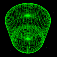
Generating Capsule GeometryWritten by Paul BourkeApril 2012
The following will briefly describe a way of creating an capsule shape, example code is supplied here: capsule.c (Tab stops to 3 spaces for correct indenting). which created the shape and saves the result as an obj file with normals and texture coordinates. The code should be easy to modify to create the mesh geometry in other formats or for APIs such as OpenGL. The output from the code plus a sample texture map are given below.
It is fairly obvious that the desired shape is just two halves of a sphere offset along the intended axis of the capsule. Also, that it is not necessary to explicitly add a central cylinder, rather just join up the equator of each half sphere. 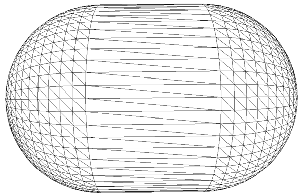
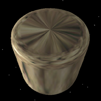
The normals are straightforward to calculate, they are just the vectors to the vertices of the normalised sphere before offsetting along the capsule axis. There are many options for the texture coordinates, the one chosen here is the projection of a sphere onto the capsule. These are computed by calculating the longitude and latitude of each vertex of the capsule and mapping those to (u,v) in the usual way. The result given the texture map (spherical projection) given above is shown below. 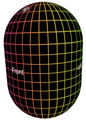
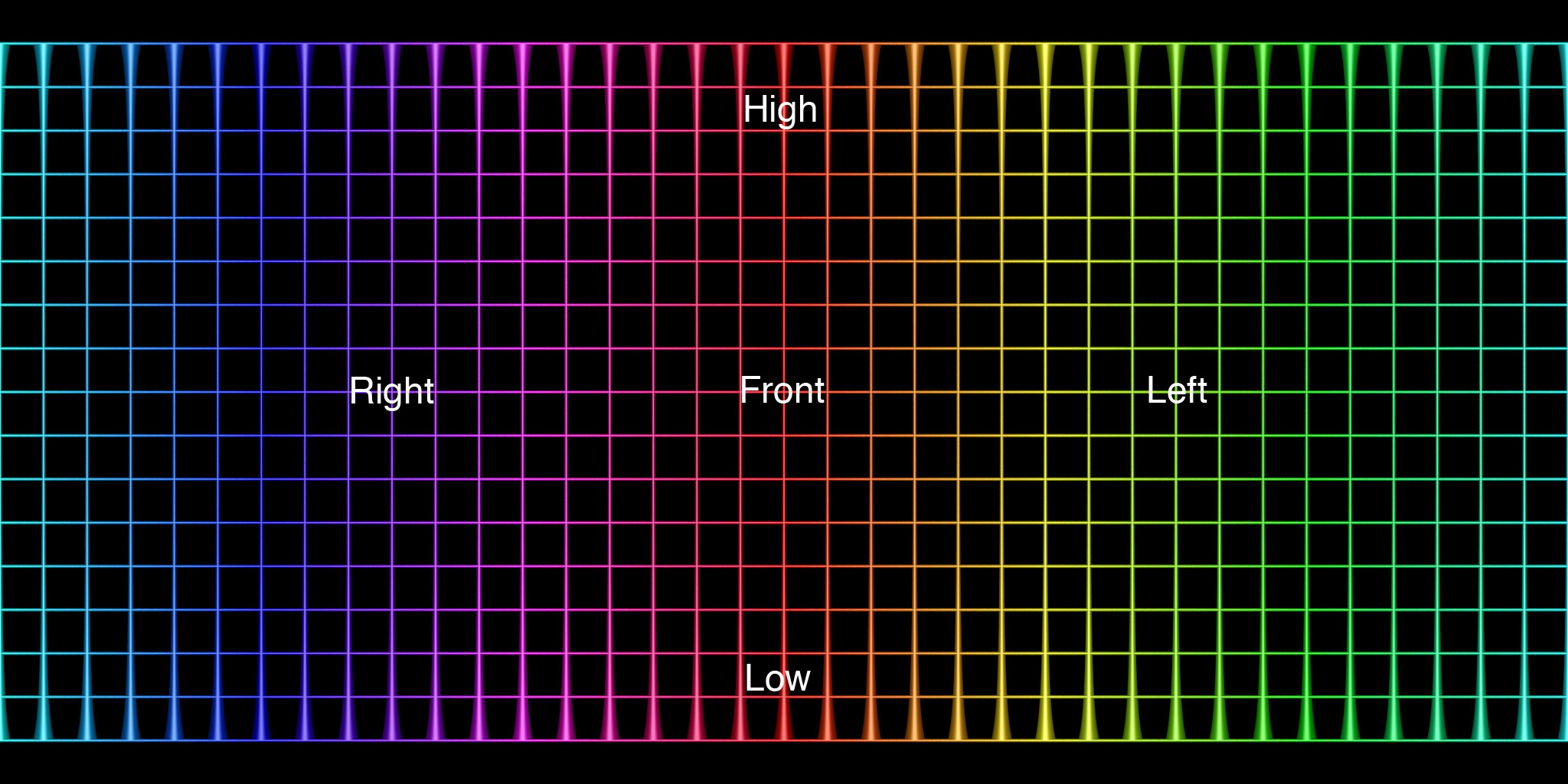
Coordinate system conventions. 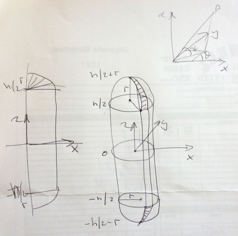
Eggs, melons, and peanuts - Cassini OvalAlso called: Cassinoid or Cassinian EllipseWritten by Paul Bourke April 2001 Introduction
Around 1680 Giovanni Cassini investigated a family of curves which he believed defined the path the Earth takes around the sun. The curves were defined by all the points where the product of the distances from the point to two fixed points (call the separation 2a) were some constant (call this b2). Note an ellipse is defined as the points where the sum of the distances to two fixed points equal some constant. The general appearance of the curve is dictated by the relative values of a and b. If a < b the curve forms a single loop, this loop becomes increasingly pinched as a approaches b. When a > b the curve is made up of two loops, at a = b it is the same as the lemnescate of Bernoulli that was documented about 14 years later. Equations
There are a number of ways to describe the Cassini oval, some of these are given below. Bipolar coordinates
Cartesian description from the definition or equivalently These clearly revert to a circle of radius b for a = 0.
Polar coordinates It is possible to solve for r2 using the standard solution for a quadratic. When using this formulation to create the curve in 2D or surfaces of revolution to form solids in 3D be very careful about the range of theta and what the positive and negative solutions mean. The parametric formulation used to create the curves and solids here is based up the following. y(t) = sin(t) sqrt(C) where C = a2 cos(2t) +/- sqrt(b4 - a4 sin2(2t))
Note:
An unexpected way to create a Cassini curve is to slice a torus with a plane parallel to the axis of the torus. As the plane is moved outwards from the centre of the torus there is a transition of Cassini curves from a > b (two loops) to a = b, and finally a < b (single loop). Examples
Sphere, a = 0.1, b = 1
Melon, a = 0.5, b = 1
Peanut, a = 0.9, b = 1
a = 0.99, b = 1
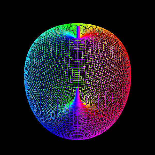
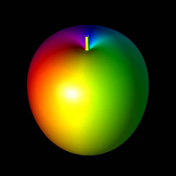
Egg, a = 1.01, b = 1
a = 1.1, b = 1
Sphere, a = 2, b = 1
Source code
The C source code that created the images on this page can be found here: cassini.c. While it creates output geometry in a particular format, the primitives are just lines and 3D polygons so it shouldn't be difficult to modify the code to create geometry in a format for your favourite package. The 3D solids are formed as surfaces of revolution about the x axis. PovRay
For PovRay users here are some examples of Cassini solids and code to create smooth triangle models: povcassini.c. The renderings here used the init file: cassini.ini and the PovRay scene file: cassini.pov. The output of povcassini.c is piped to "cassini.inc".
Ellipse
Kissing NumberWho said geometry wasn't romantic?
Written by Paul Bourke
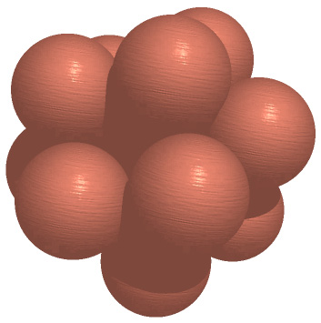
The so called "kissing number" is the maximum number of times a sphere in N dimensional space can touch a central sphere (all spheres are the same size and cannot intersect another sphere). 2DConsider the situation in 2 dimensions, a 2D sphere is just a circle and it is easy to verify that the kissing number is 6. That is, at most 6 circles of equal radius can be packed around a central circle of the same radius....try it with 7 coins all of the same denomination! 
The one dimensional case is rather boring with a kissing number of 2. 3DIn 3 dimensions the kissing number is 12, this can be verified with ping-pong balls and bits of masking tape to hold them together. There is more than one way to pack the 12 spheres, the example below is a very symmetric solution. Another method is to arrange the spheres so their centers lie along at the vertices of an icosahedron. There does seem to be lots of "empty" space but there isn't enough for another sphere! 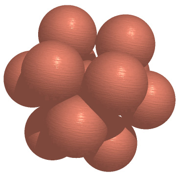
For a slightly more non-symmetric example see the following coordinates (center of each kissing sphere) and corresponding image.
          x            y            z
     0.25531102   0.89156330  -0.37407374
    -0.13044368  -0.77593450  -0.61717914
     0.12484695   0.78152529   0.61125401
     0.79480098  -0.47827054  -0.37356217
     0.45181161  -0.14070529   0.88094738
     0.91933526   0.36212485   0.15390992
     0.21657532  -0.92622152   0.30855928
    -0.91836971  -0.36091967  -0.16227776
    -0.62695983   0.48432758  -0.61020338
    -0.79681573   0.47329850   0.37559716
     0.22672985   0.08894927  -0.96988742
    -0.51617898  -0.41001744   0.75196074
The kissing number is known for certain for many higher dimensions and suspected for others. The table below gives the values for a range of dimensions. In the cases where the maximum hasn't been proved the number below has generally be determined by exhaustive computer searches. The exact value for 24 dimensions was found in 1979 by A.M. Odlyzko and N.J.A. Sloane. Dimension Kissing Number 1 2 2 6 3 12 4 24 5 at least 40 at most 44 6 at least 72 at most 78 7 at least 126 at most 134 8 240 9 at least 306 at most 364 10 at least 500 at most 554 11 at least 582 at most 870 12 at least 840 at most 1357 13 at least 1130 at most 2069 14 at least 1582 at most 3183 15 at least 2564 at most 4866 16 at least 4320 at most 7355 17 at least 5346 at most 11072 18 at least 7398 at most 16572 19 at least 10688 at most 24812 20 at least 17400 at most 36764 21 at least 27720 at most 54584 22 at least 49896 at most 82340 23 at least 93150 at most 124416 24 1965604D For those with an interest in 4D geometry, here are the coordinates for a solution with 24 kissing hyperspheres.
          x            y            z            w
     0.75380927  -0.28878253  -0.17107694  -0.56489726
    -0.75380927   0.28878253   0.17107694   0.56489726
     0.00158908   0.23980955  -0.40088438  -0.88418356
     0.88625386   0.32965258  -0.25236023   0.20542051
     0.33787744  -0.01190412  -0.92962202  -0.14662890
     0.41593183  -0.27687841   0.75854507  -0.41826836
     0.13403367   0.85824466  -0.48216766  -0.11386579
     0.33628835  -0.25171367  -0.52873764   0.73755466
     0.54837642   0.34155670   0.67726179   0.35204941
    -0.33628835   0.25171367   0.52873764  -0.73755466
     0.20384377  -0.87014878  -0.44745436  -0.03276311
     0.13244459   0.61843511  -0.08128328   0.77031777
    -0.41593183   0.27687841  -0.75854507   0.41826836
     0.75222019  -0.52859208   0.22980744   0.31928630
    -0.13244459  -0.61843511   0.08128328  -0.77031777
    -0.88625386  -0.32965258   0.25236023  -0.20542051
    -0.54837642  -0.34155670  -0.67726179  -0.35204941
    -0.20384377   0.87014878   0.44745436   0.03276311
    -0.54996550  -0.58136625  -0.27637741   0.53213415
    -0.13403367  -0.85824466   0.48216766   0.11386579
     0.54996550   0.58136625   0.27637741  -0.53213415
    -0.00158908  -0.23980955   0.40088438   0.88418356
    -0.75222019   0.52859208  -0.22980744  -0.31928630
    -0.33787744   0.01190412   0.92962202   0.14662890
 Represented in Second Life

Equirectangular projection
|


