Representations of laser scan dataWritten by Paul BourkeDecember 2015
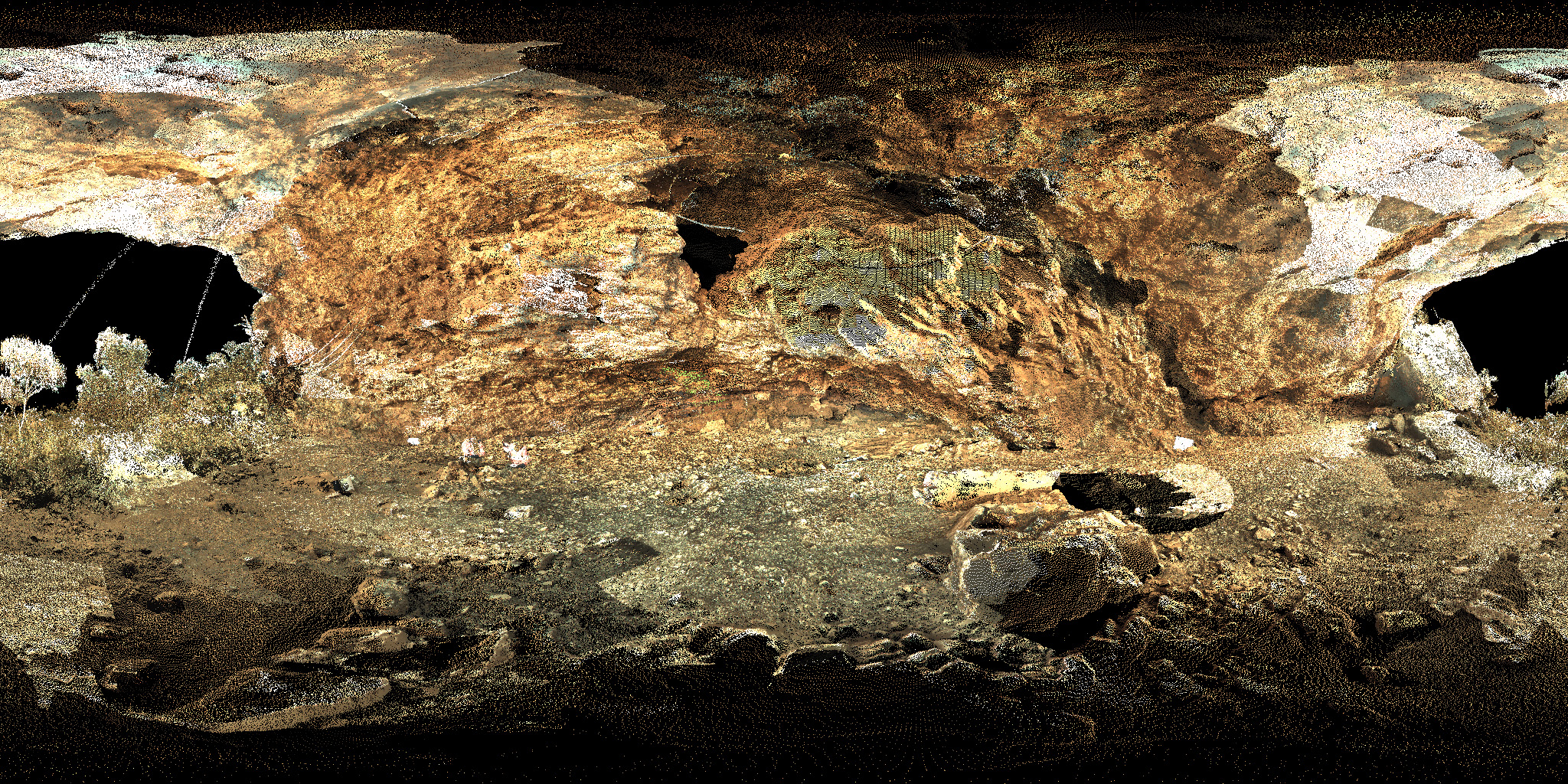
The following is some experimentation around representations of laser scan data in a format that might suite virtual environments, and in particular HMD devices. The approach is to render into spherical projections, also known as equirectangular projections. The key characteristic of this projection is that it represents everything that is visible from a single position, that is 360 degrees of longitude and 180 degrees of latitude. In the case of point clouds from a laser scanner, every point is potentially represented in the image. The datasets used here were acquired by Spatial Sciences at Curtin University on behalf of Rio Tinto and Rock Art Archaeology at The University of Western Australia. For more information see A Methodological Case Study of High Resolution Rock Art Recording in the East Pilbara, Western Australia. Example 1Leica ScanStation C10 88 million points + RGB values In the case of the first two examples from the Leica ScanStation C10 the rendering is a depth base one. That is, for each pixel the projection into the spherical image is updated only if it is the closest point to the virtual camera. This is similar to the so called z-buffer rendering for real time APIs such as OpenGL. 
The Leica C10 includes a co-registered camera to give RGB estimates at each point. However the density used in these scans is so low as to limit the application for direct viewing within an immersive display. While these spherical projections are only 2Kx1K pixels there aren't enough points to form a really "solid" surface, unless perhaps one views them from the position of the scanner. 
In all cases here multiple stations were chosen in an attempt to maximise the coverage of theses relatively convoluted rock shelters. When using a conventional perspective camera and viewing the structures from or close to the capture positions the coverage looks good, in reality there are still lots of unscanned locations and shadow zones. Example 2Leica ScanStation C10 200 million points + RGB values

Example 3
In the following three examples from the Trimble TX5 scanner there is no RGB colour information for every point, but in compensation there is almost an order of magnitude more points. The effective representation of these point clouds requires a bit more imagination to avoid simply getting solid white blobs. The rendering approach here projects each scanner point onto the spherical image plane with a 1/(distance from the camera) weighting. The effect of this is to provide some curvature information for surface parallel to the camera view. 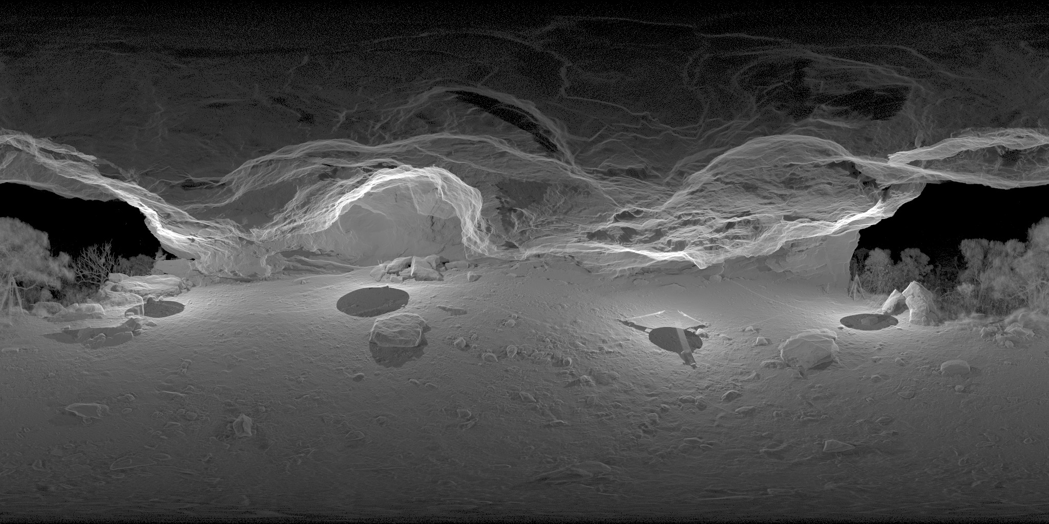
The circular patches on the ground are the unscanned region below each station location. While the circle may get scans from adjacent station locations the density is much lower overall. The other noticeable effect is the "thinning" of density towards the top and the bottom of the image, the same distortion that occurs on a Earth map towards the north and south poles. This is only a perceived thinning due to the nature of a spherical projection, within a look-around style HMD there is no density thinning. 
Example 4
These renditions of the point cloud, I claim, are beautiful. Ghostly images where the curvature of the underlying geometry is created by the addition of "in line of sight" contributions. The approach is similar to how many astronomical datasets are rendered, in that case if light is being added along the pixel wedges then it make more sense. In this case one can end up seeing structure that would normally be obscured behind other solid structure. 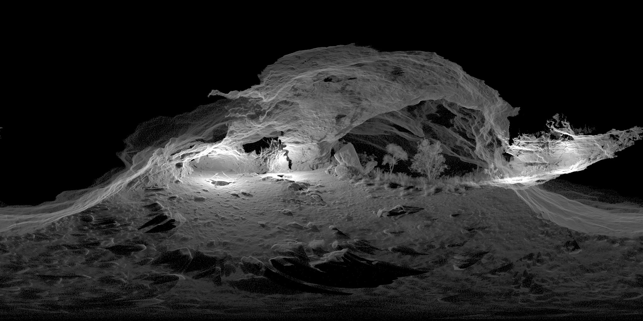
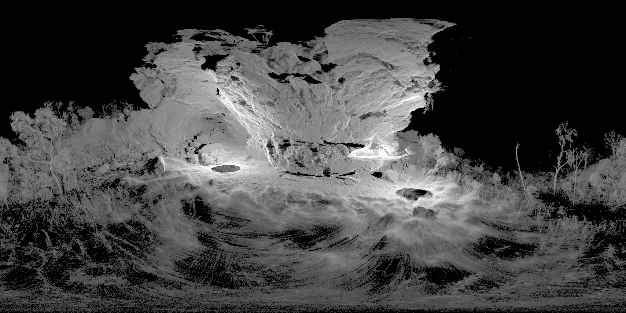
Example 5 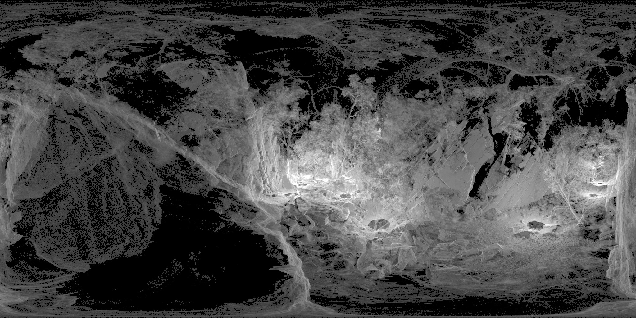
Notes
|