Workflow for comparing two photogrammetrically reconstructed meshesWritten by Paul BourkeJanuary 2015
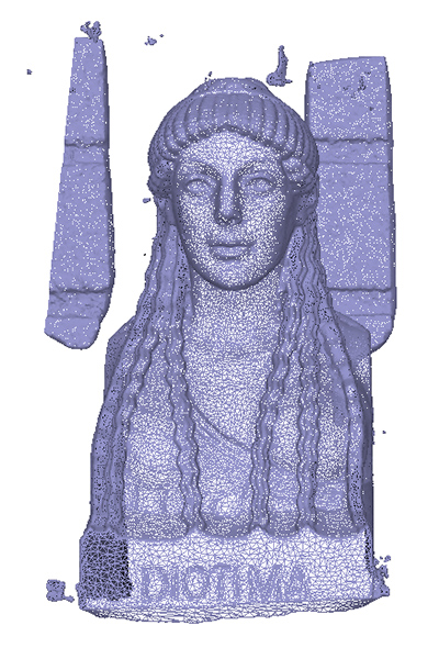
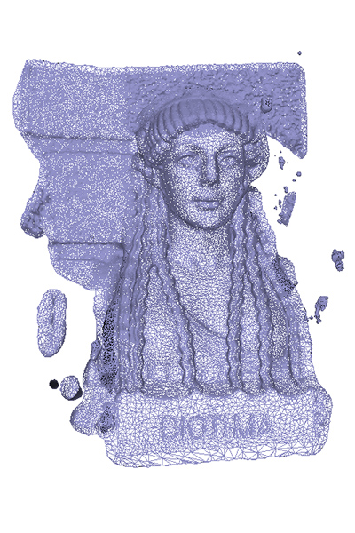
The following describes one possible pipeline for comparing two point clouds (or meshes) using the "CloudCompare" software. The particular application in mind is comparing multiple photogrammetric reconstructions for the purpose of estimating repeatability error or for comparing point clouds derived from laser scans with photogrammetric reconstructions. As with many guides relating to software implementations it can go out of date as new versions of the software are released. This document is based upon version 2.6 of CloudCompare, version 1.1.0 of PhotoScan, and version 1.3.3 of MeshLab. For the purposes of this document we will compare two meshes derived from only a set of 11 photographs. These are split into two sets (6 even and 5 odd numbered photographs) and each reconstructed independently. For this exercise PhotoScan is used, both sets of images processed through the same batch processing steps. In general such reconstructions, without markers and calibrated cameras will be of arbitrary scale and orientation. In most cases, but not here because of the small number of non-optimal photographs in the second set, there is not expected to be differential axis scaling.
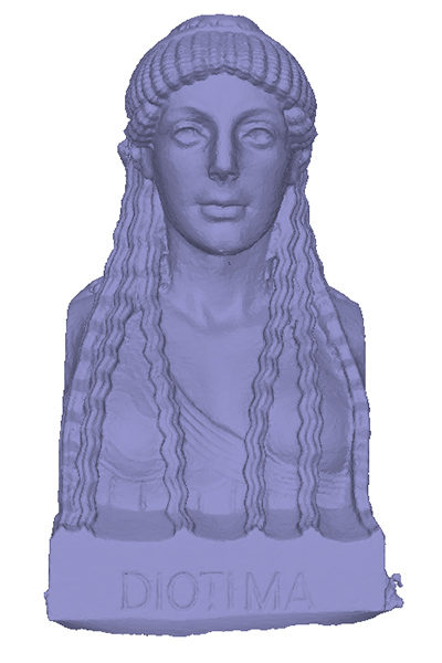
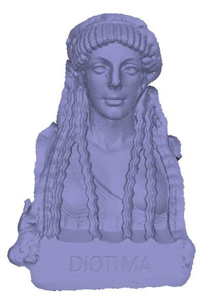
In order not to complicate the alignment and interpretation of the comparison the extraneous parts of the mesh should be removed. This cleaning process can be performed within PhotoScan itself or within MeshLab. The resulting mesh data shown below also highlights that in this case the model is stretched in one axis, arising from the low number of photographs from the second set resulting in a distorted and more noisy mesh. The author generally saves textured meshes in OBJ format, simple human readable format with wide support. A number of export formats from MeshLab can be used to take the mesh or just the points into CloudCompare, but OBJ is also recommended.
Opening the two meshes in CloudCompare is shown below, note the two models are in different coordinate systems, see yellow bounding boxes. 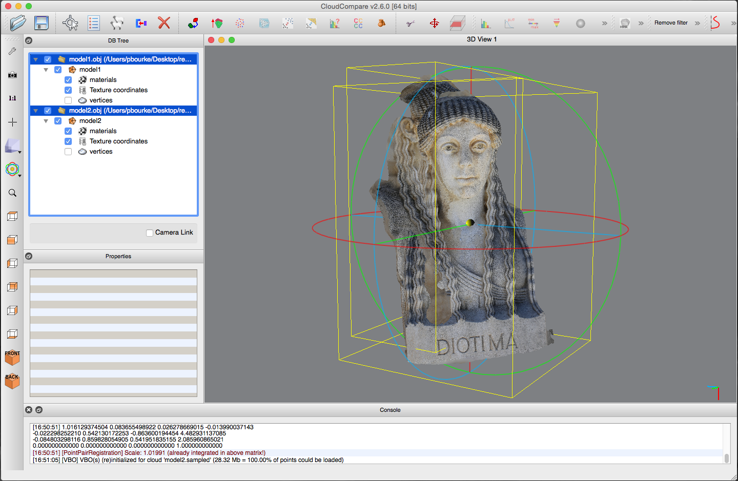
Since, as the name suggests, CloudCompare is designed to compare two point clouds, as such the meshes need to be represented by points. There are a number of ways of doing this, for dense meshes the mesh vertices themselves may be sufficient. Otherwise CloudCompare offers methods for sampling the surfaces of the meshes to create an arbitrary dense point cloud. The meshes should be sampled to a convenient resolution for picking corresponding points in the next step, generally between 1 and 2 million points, see menu "Edit" -> "Mesh" -> "Sample points". It is recommended that colour information from the mesh texture maps is applied to the points, this greatly assists the corresponding point selection. 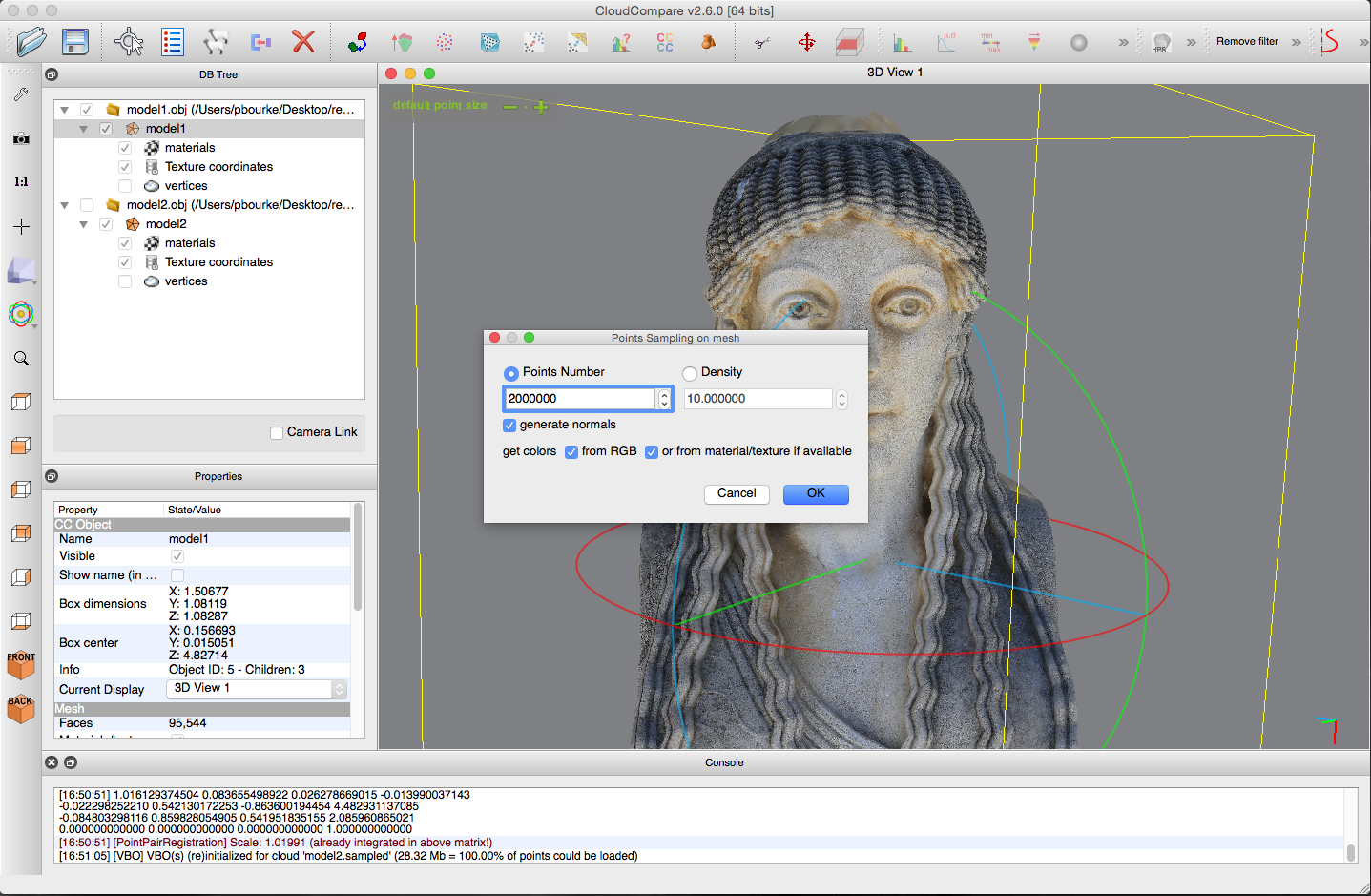
The two resulting sampled meshes are shown below, the two coordinate systems are obvious. While the intent here is not to describe the CloudCompare interface in detail, note that mesh and point cloud assets can be selected/deselected, made visible/invisible using the check boxes in the "DB Tree" window. 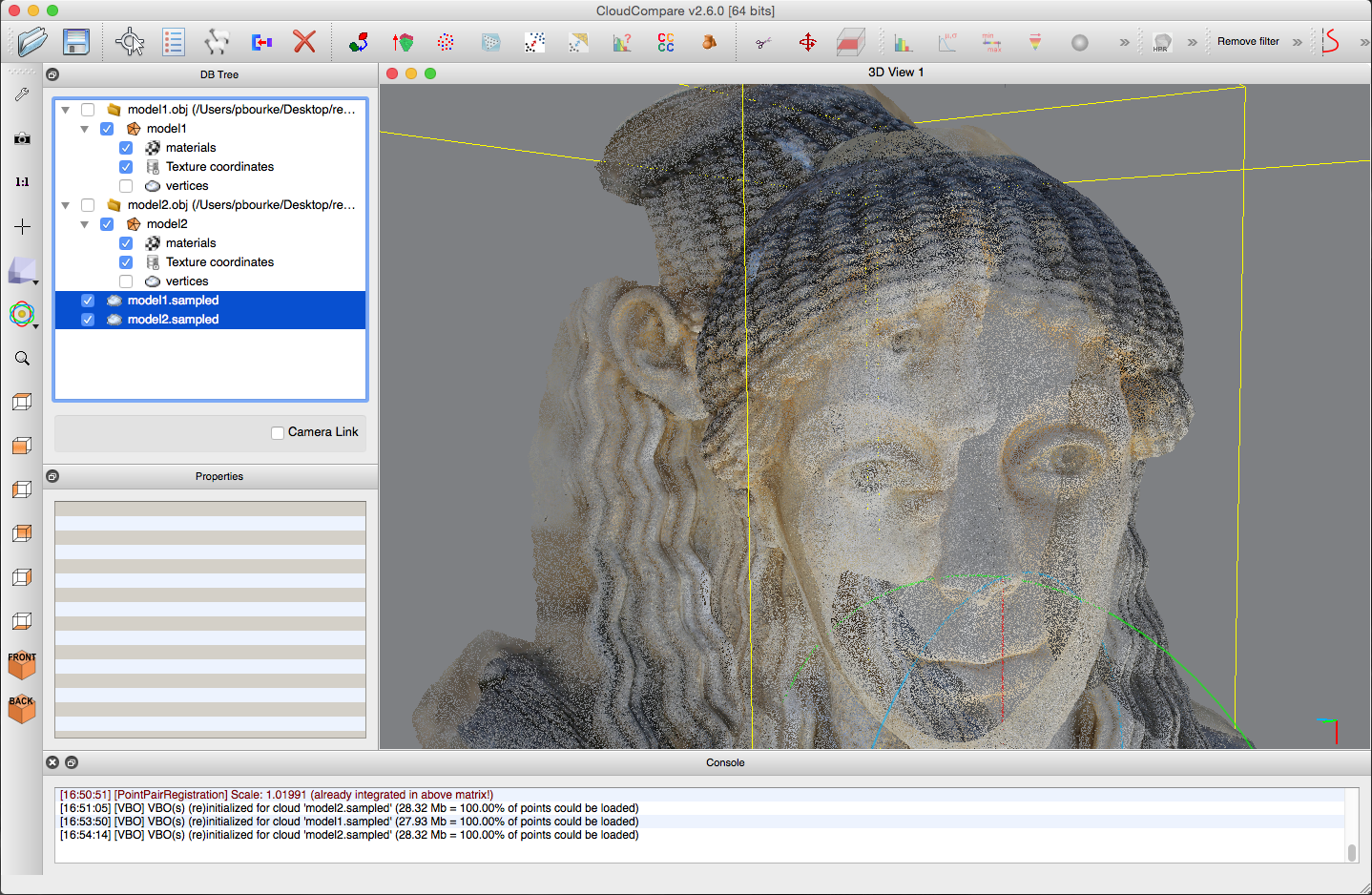
Before a comparison can be performed the two meshes need to be aligned to the same coordinate system. CloudCompare offers a number of methods to achieve this depending on the characteristics of the two point clouds to be compared. One may align manually, align the bounding boxes, automatic alignment, or perform alignment based upon manually chosen corresponding points in each point cloud. The later approach will be recommended here, it does generally rely on point clouds with RGB values to assist with the selection of corresponding points. Select the "Align two clouds" icon from the tool bar. It is necessary to select one point cloud as the reference, the coordinate system of this point cloud will not be changed, the coordinate system of the other point cloud will be modified by a general 4x4 matrix to bring it into the closest coordinate system of the reference. 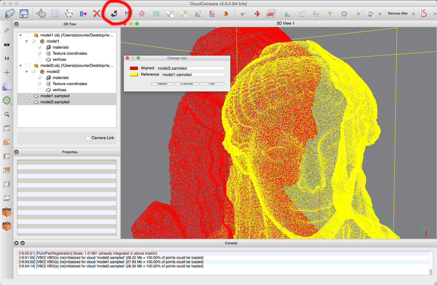
By alternatively selecting one point cloud and then the other, select at least 4 corresponding points on each point cloud. Better results will be achieved if the points span depth in all three axes. For example, relatively poor alignment can result if the points are almost co-linear or co-planar. 6 coincident points in the reference cloud are illustrated below. 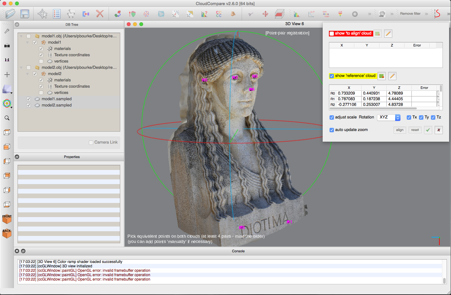
It is obviously critical that the points are selected in the same order in each point cloud. A1 (Align point 1) must refer to the point R1 (reference point 1). The following shows both point clouds and the corresponding points on each. 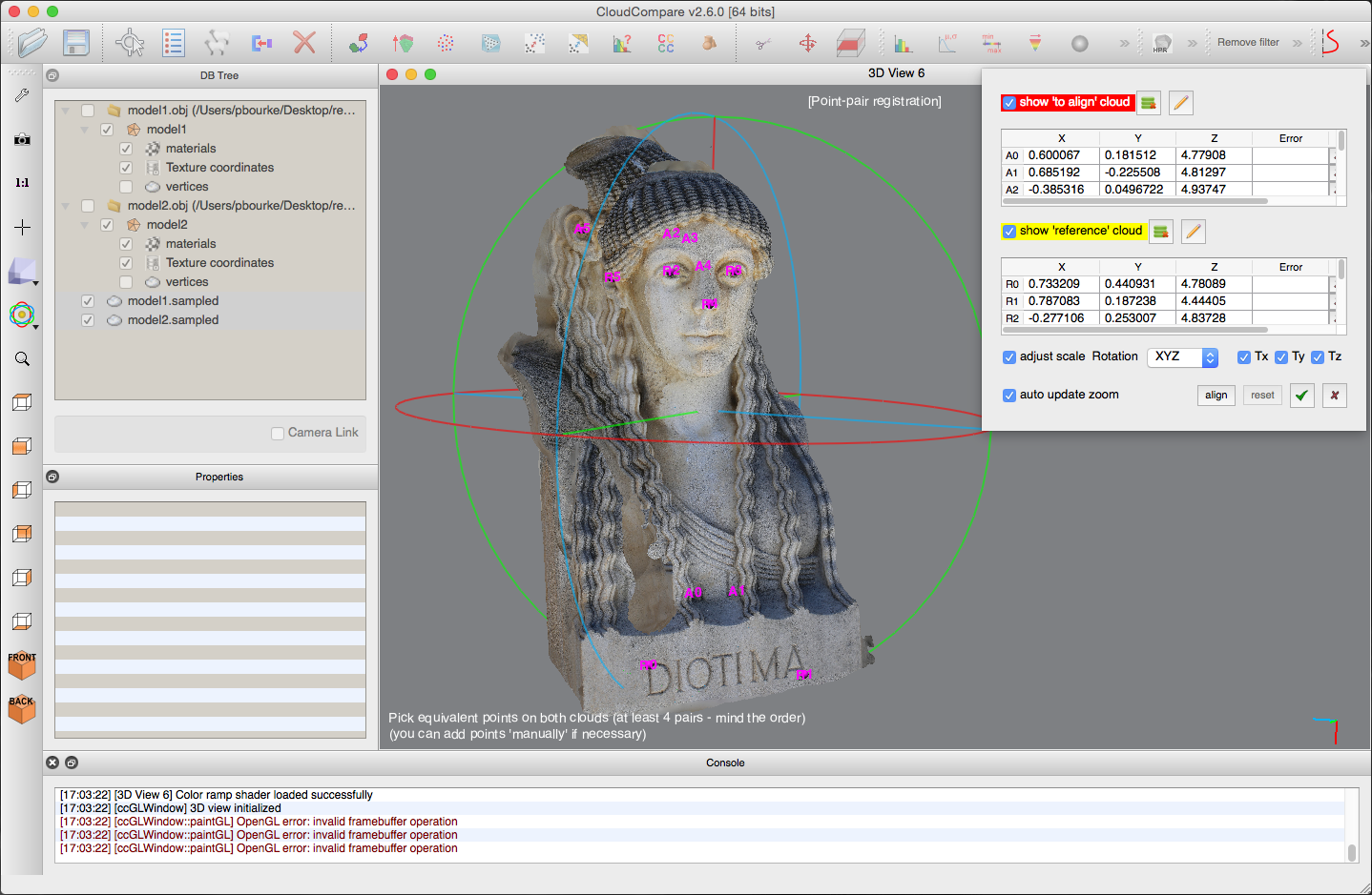
In this case the alignment includes scaling, as well as more usual normal translation and rotations. If the purpose was to determine if there were any differential scaling between sets then this option can be removed from the alignment options. The following shows the aligned meshes. Note that while the yellow bounding boxes don't coincide, they are parallel to each other indicating there is only a difference in the extent of the mesh reconstructed. A note to more advanced use: the 4x4 rigid transformation matrix is provided and can be selected/copy/pasted and thus applied to other meshes in CloudCompare. For example one might align a small part of an overlapping point cloud and then apply the 4x4 matrix to a point cloud or mesh of larger extent. 
There are a number of metrics that can be computed in Cloud Compare. Perhaps the most common is the "cloud to cloud" distance, see tool bar. 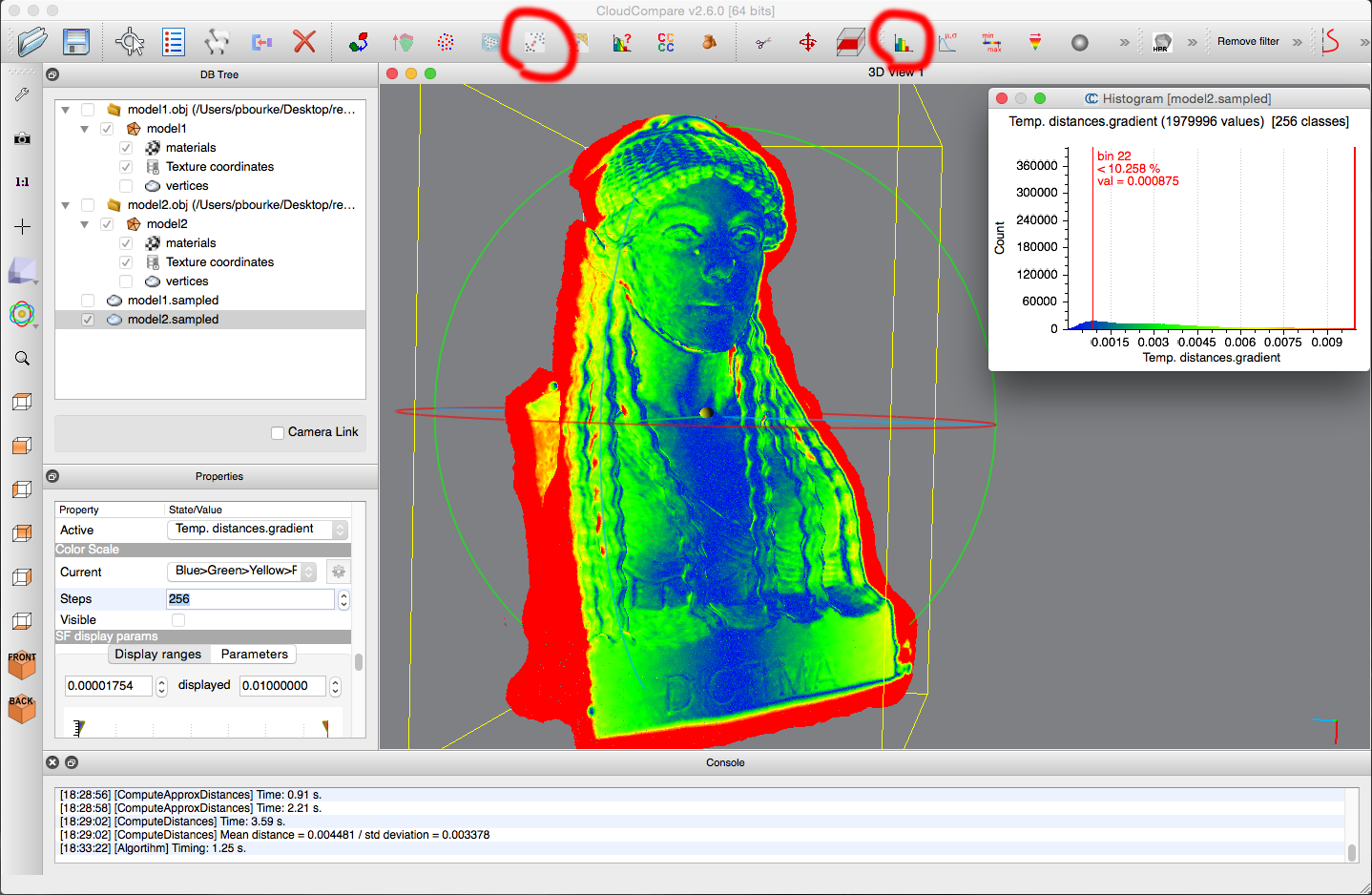

If the intent was to create statistics based upon real world units (normally the case) then one should scale the models based upon a known distance, or measure a known distance and apply the scaling to the subsequent statistics. One way to do this in CloudCompare is to measure a known distance, in this case the distance between the eyes is 0.10m. The point cloud can then be scaled using the "Edit" menu- > "Multiply/Scale" option. 
|