Report: Enhancing rock art recordings through multispectral photographyWritten by Paul BourkeOctober 2014 See Thai translation courtesy of Ashna Bhatt.
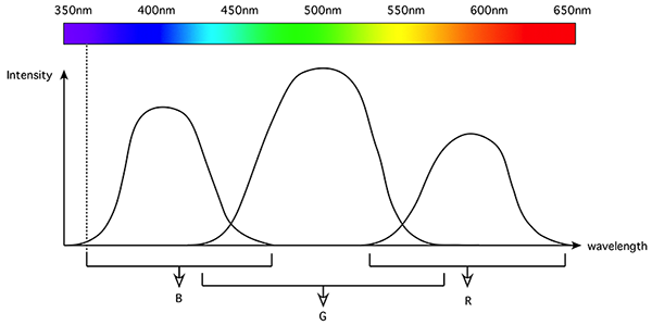
The following is an initial investigation into using multispectral photography (also often referred to as multispectral imaging) to enhance difficult to identify indigenous Australian rock art. The use here of the term multispectral is taken to mean photography at narrow frequency bands across the visible spectrum. This is motivated by the realisation that a digital camera, and also the human eye, integrates the wavelengths over three channels (red, green, blue) to produce a single RGB value for each pixel. As such a large amount of information is being lost, namely the intensity of any particular wavelength. Some of the consequences are:
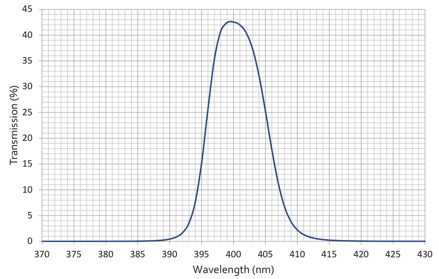
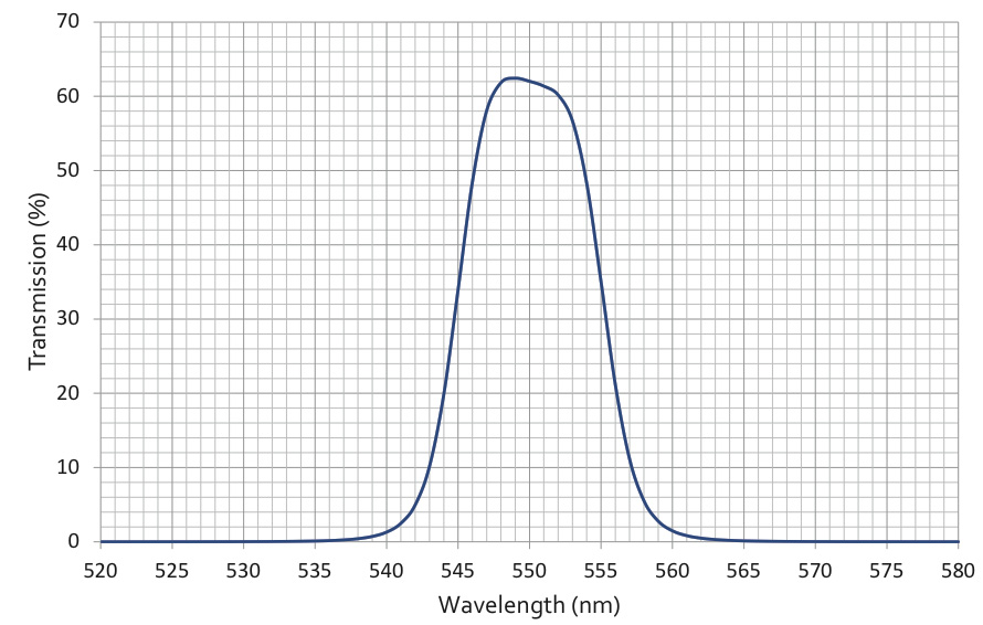
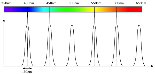
The ultimate in multispectral recordings might be to capture the intensity continuously across some wavelength range resulting in a wavelength signature. This is being used in a number of industries, for example, to identify minerals in mining exploration. An approximation is to integrate the electromagnetic intensity over a number of narrow wavelength bands. The result of a multispectral image is often referred to as a spectral cube, that is, for each pixel (x,y) in the image there is some wavelength (λ) intensity value. This dataset is then imagined as a cube of (x,y,λ). For a usual RGB image there are only three slices of this cube in the wavelength dimension, and they are not necessarily independent or of narrow extent in λ. For the example discussed here there are possibly 8 slices captured in the wavelength dimension, each slice is non-overlapping (independent). Multispectral imaging can be very precise with calibrated equipment and response curves for the entire processing pipeline. For the purposes here the intent is more qualitative, that is, to identify and reveal further structures in otherwise indistinct rock art. The filters selected for this test were precise interference bandpass filters spanning the visible electromagnetic spectrum. Interference bandpass filters, rather than absorbing unwanted wavelengths, reflect them. Filters were chosen at 50nm steps across the visible spectrum, from 350nm to 700nm (due to availability the highest wavelength was actually 690nm). The filters all had a full width half maximum (FWHM) of 10nm, and are supplied with known measured response curves, two examples of which are shown below. As such, there is no overlap between the bandpass centers chosen and therefore each captured image is wavelength independent of its neighbours.
The filters are available (Knights Optical, UK) in a range of diameters. The largest available 50mm diameter was chosen in order to support a large lens diameter. Given the low light energy collected across a narrow 20nm band, a large collecting area will maximise the opportunity for short exposure times. A 50mm prime lens (1:1.8) was chosen mainly because it allowed the filters to sit on the lip in the front of the 52mm thread. 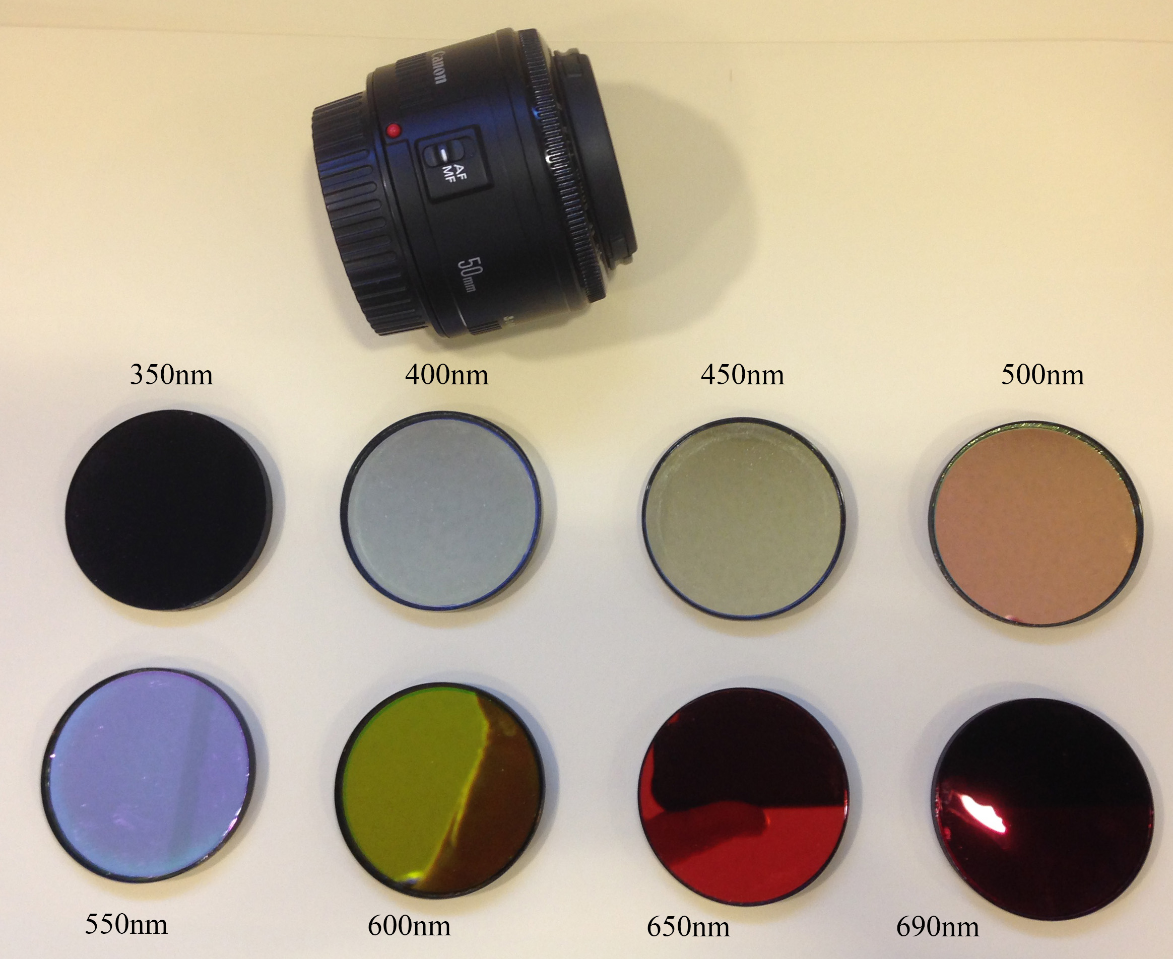
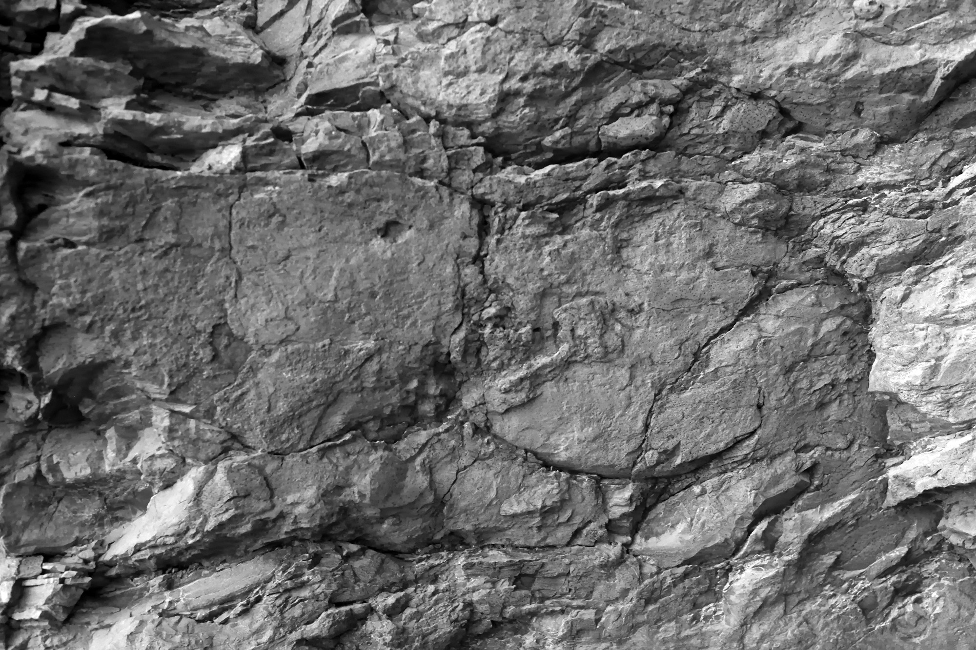
The following photograph is an unmodified image off the camera (Canon 5D Mk III) of an approximately 1m wide rock with vaguely visible vertical lines (clearer in real life with particular sun illumination). 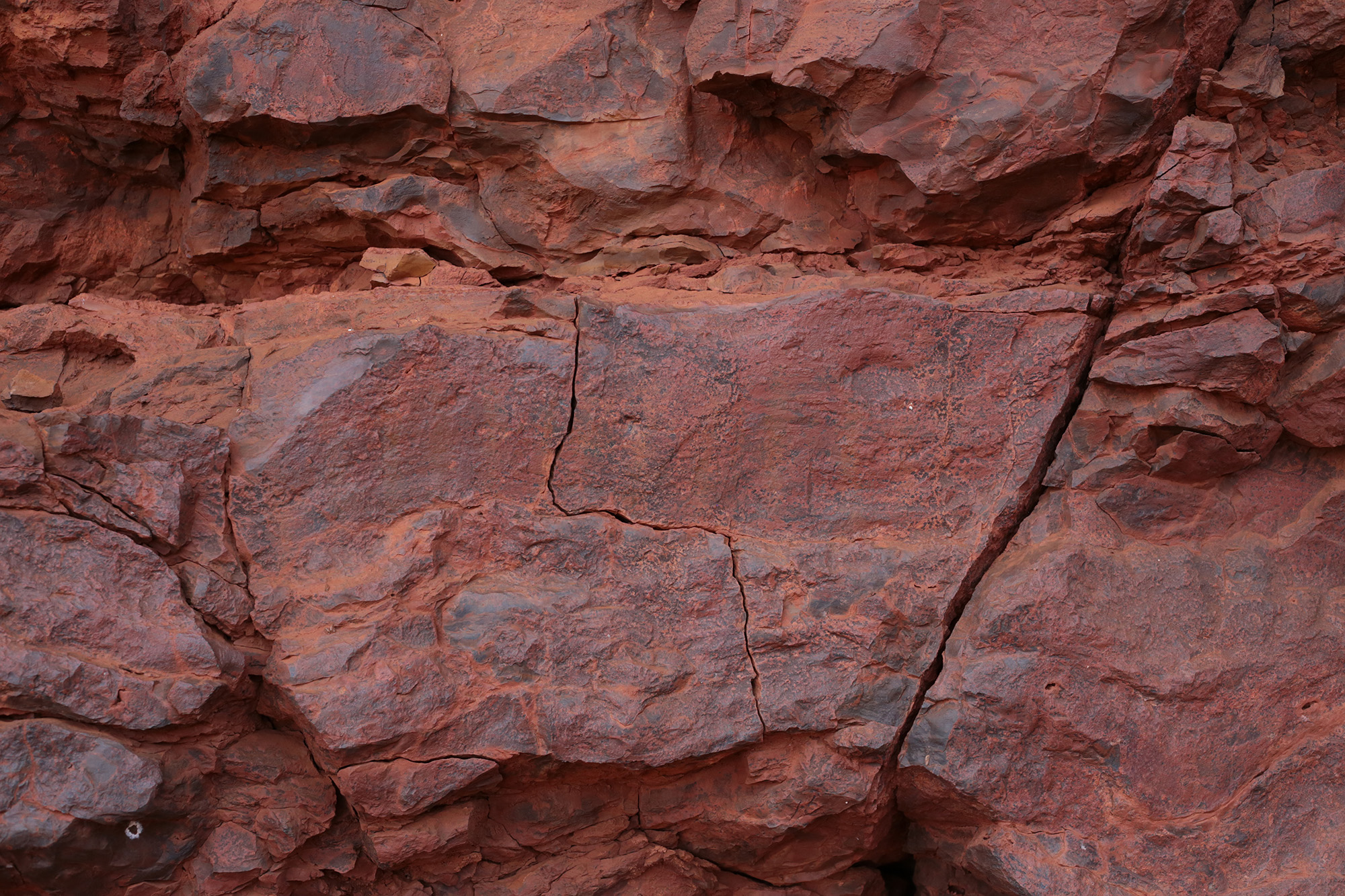
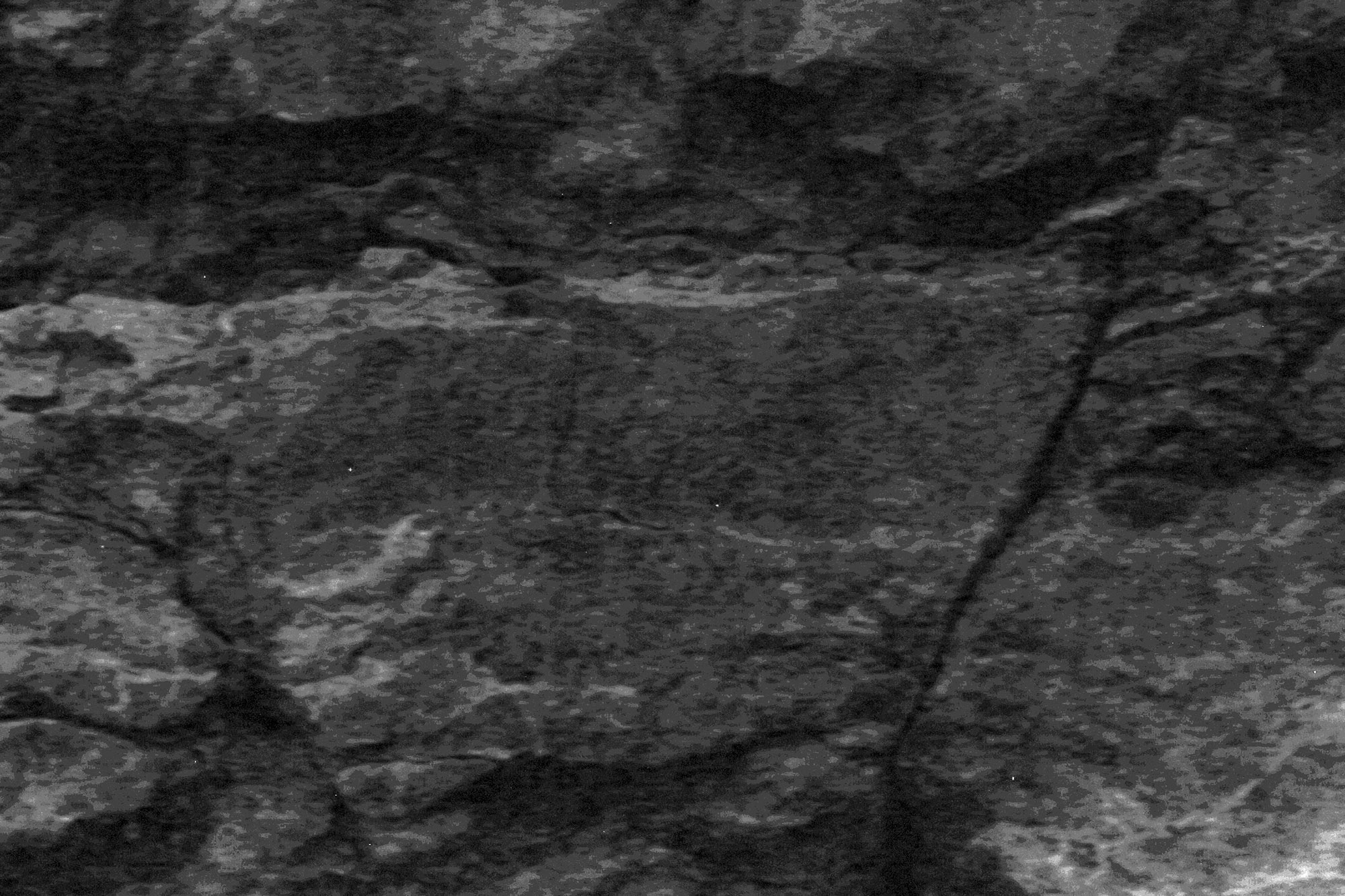
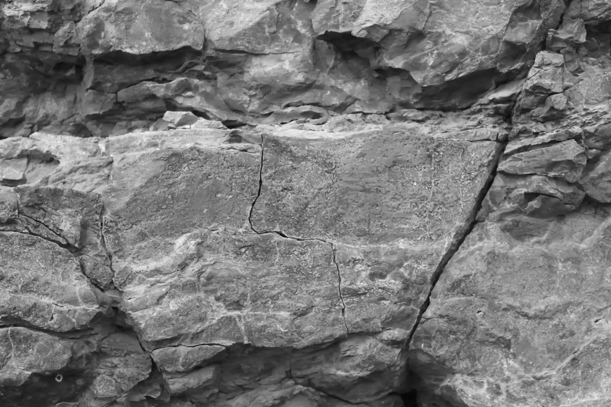
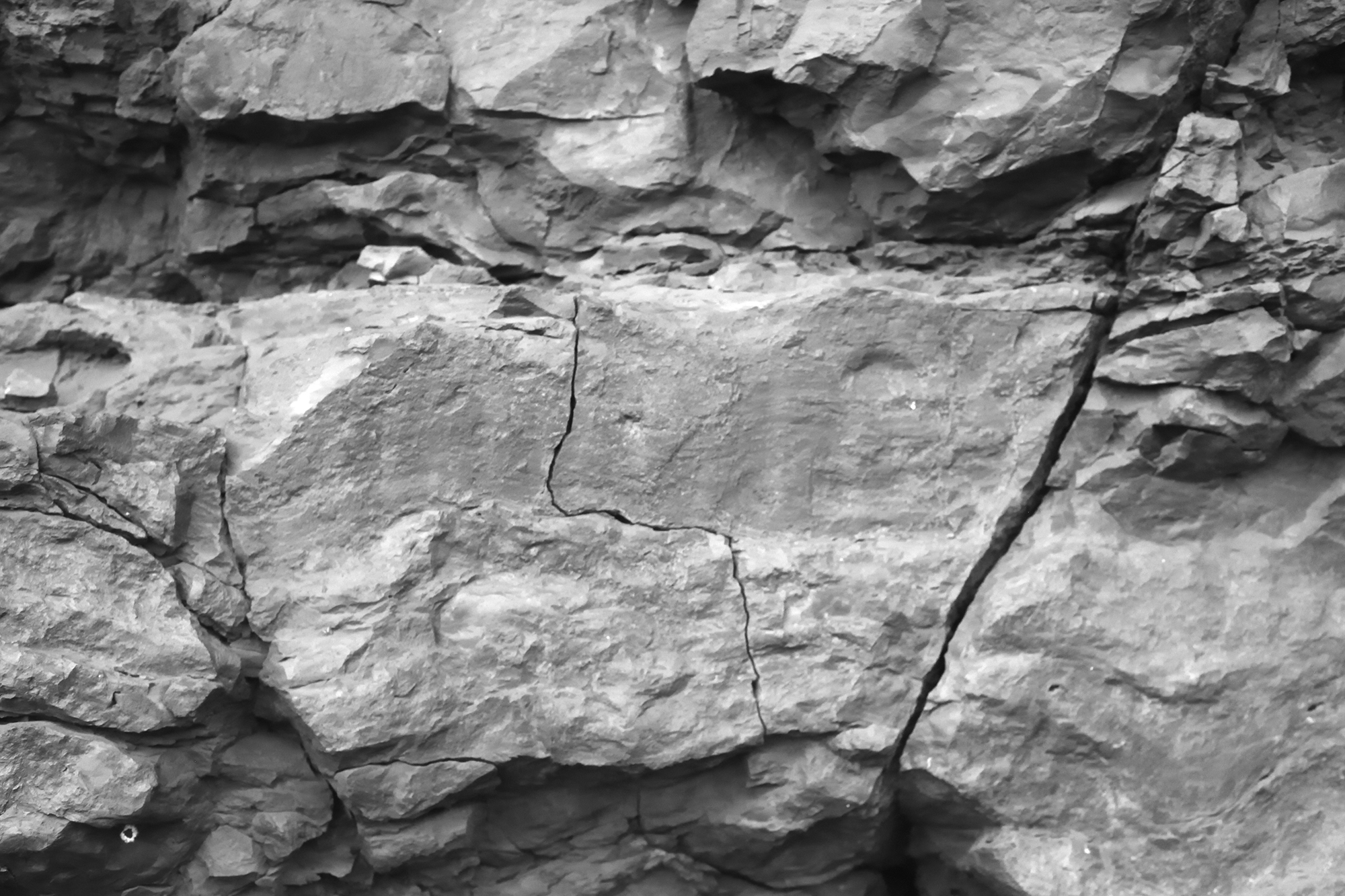
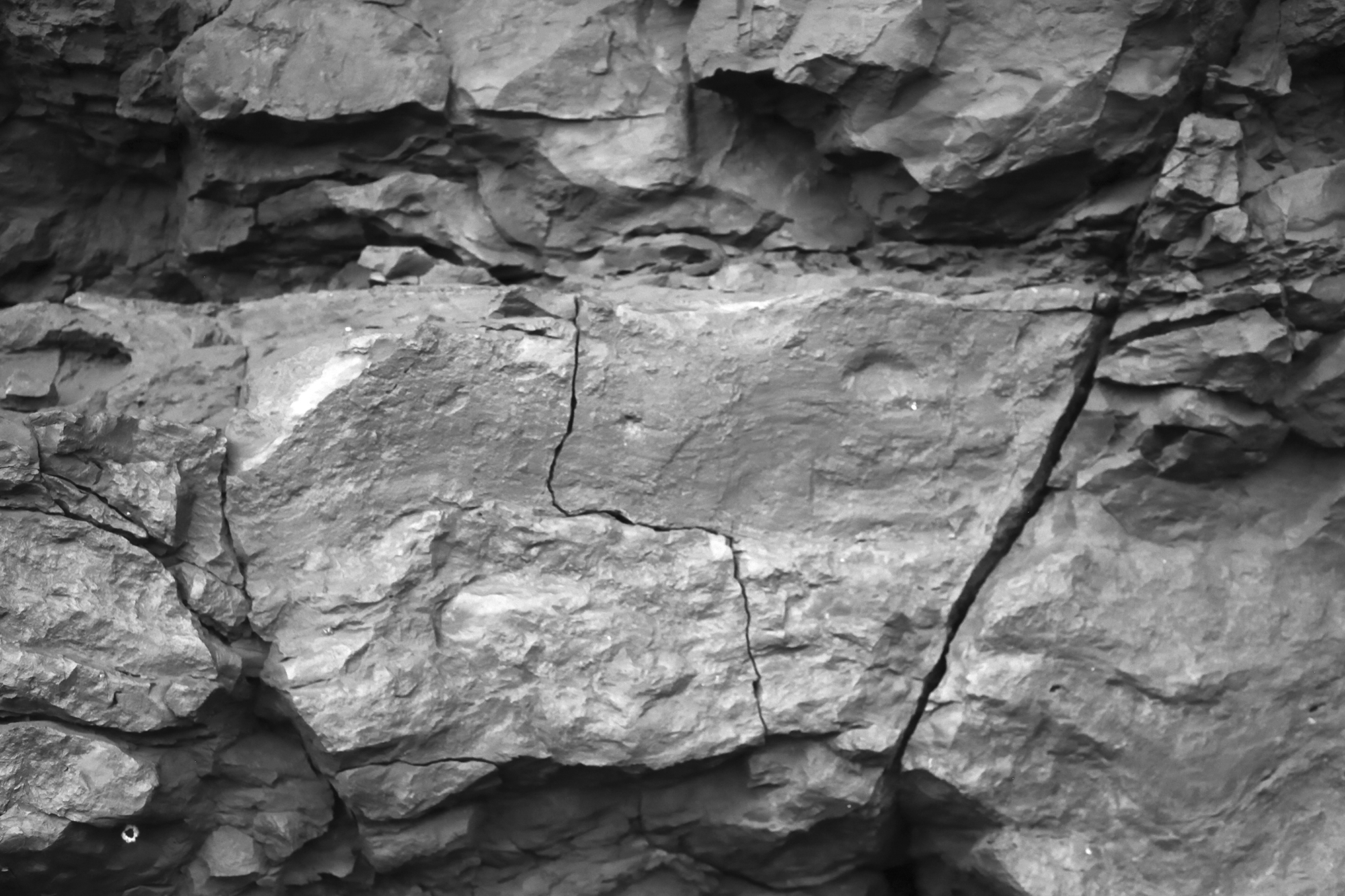
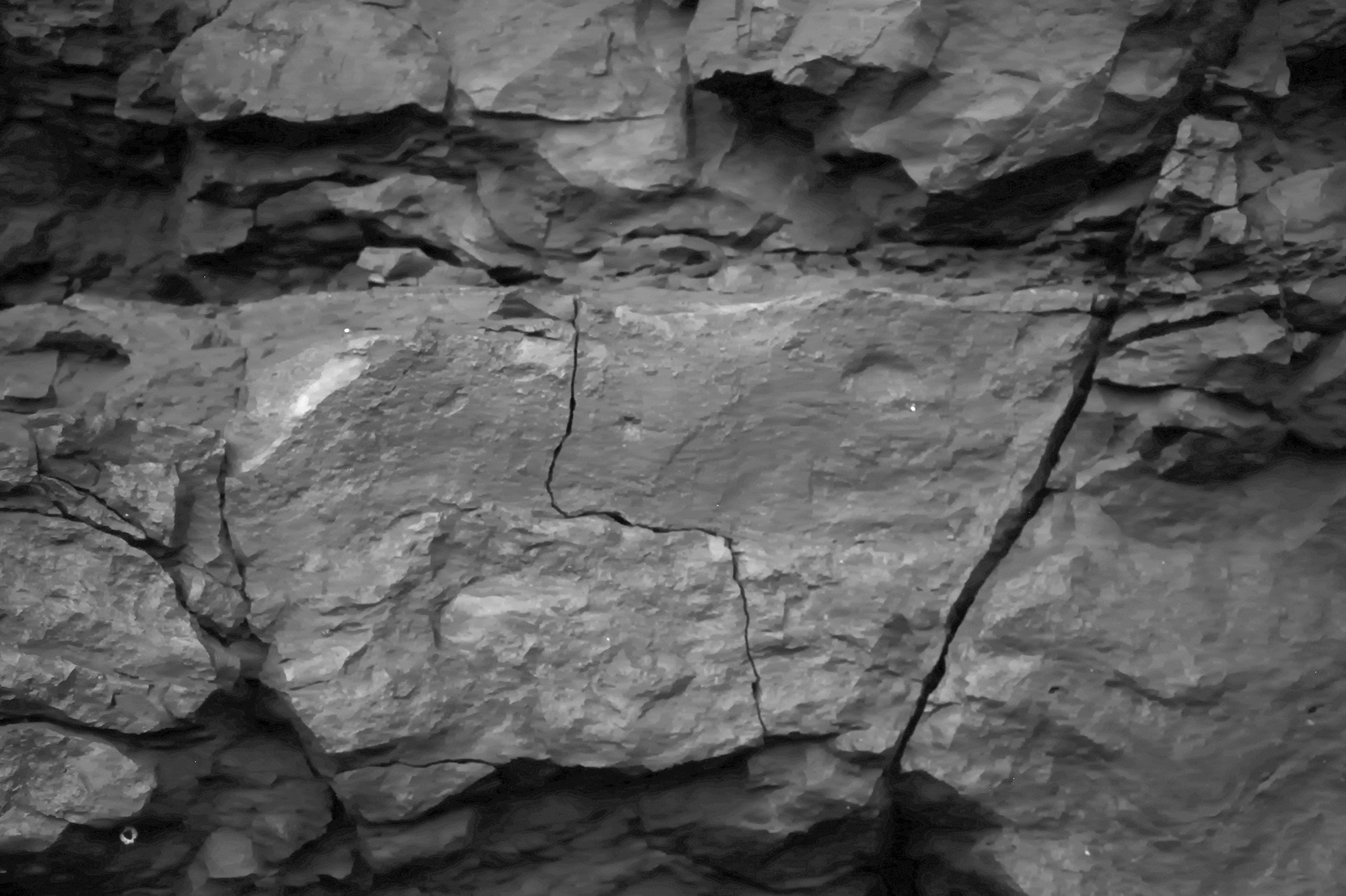
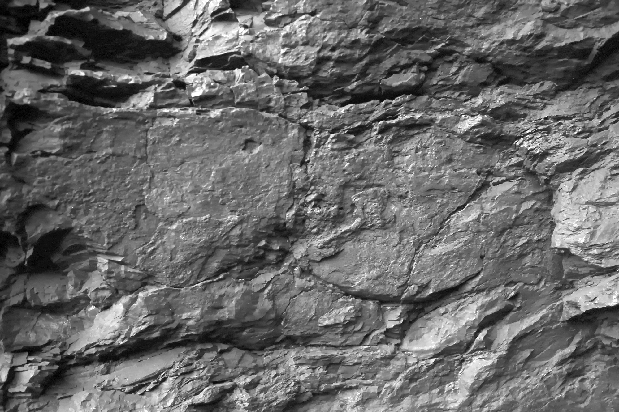
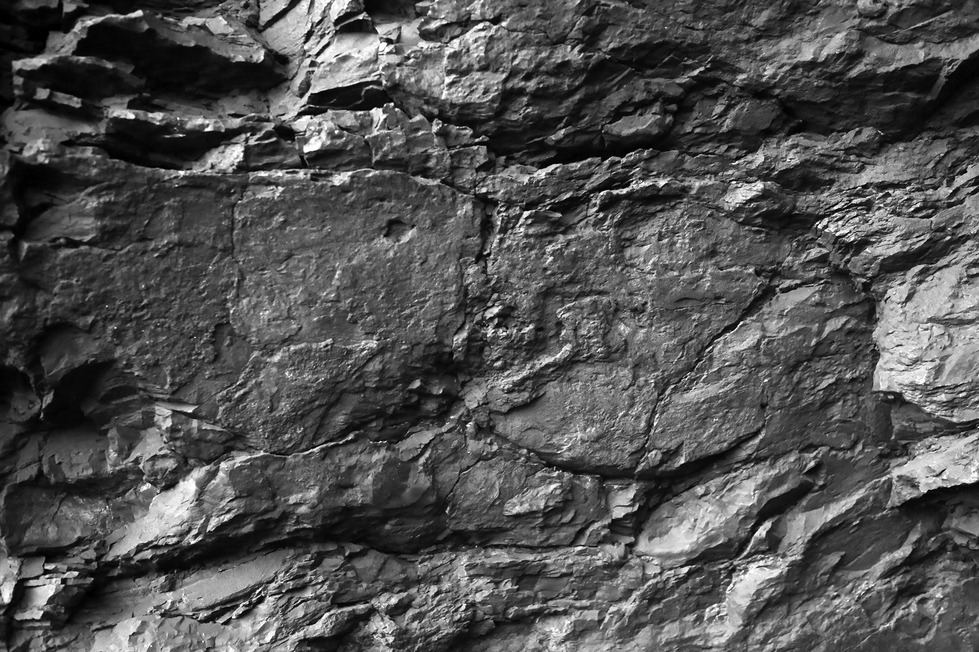
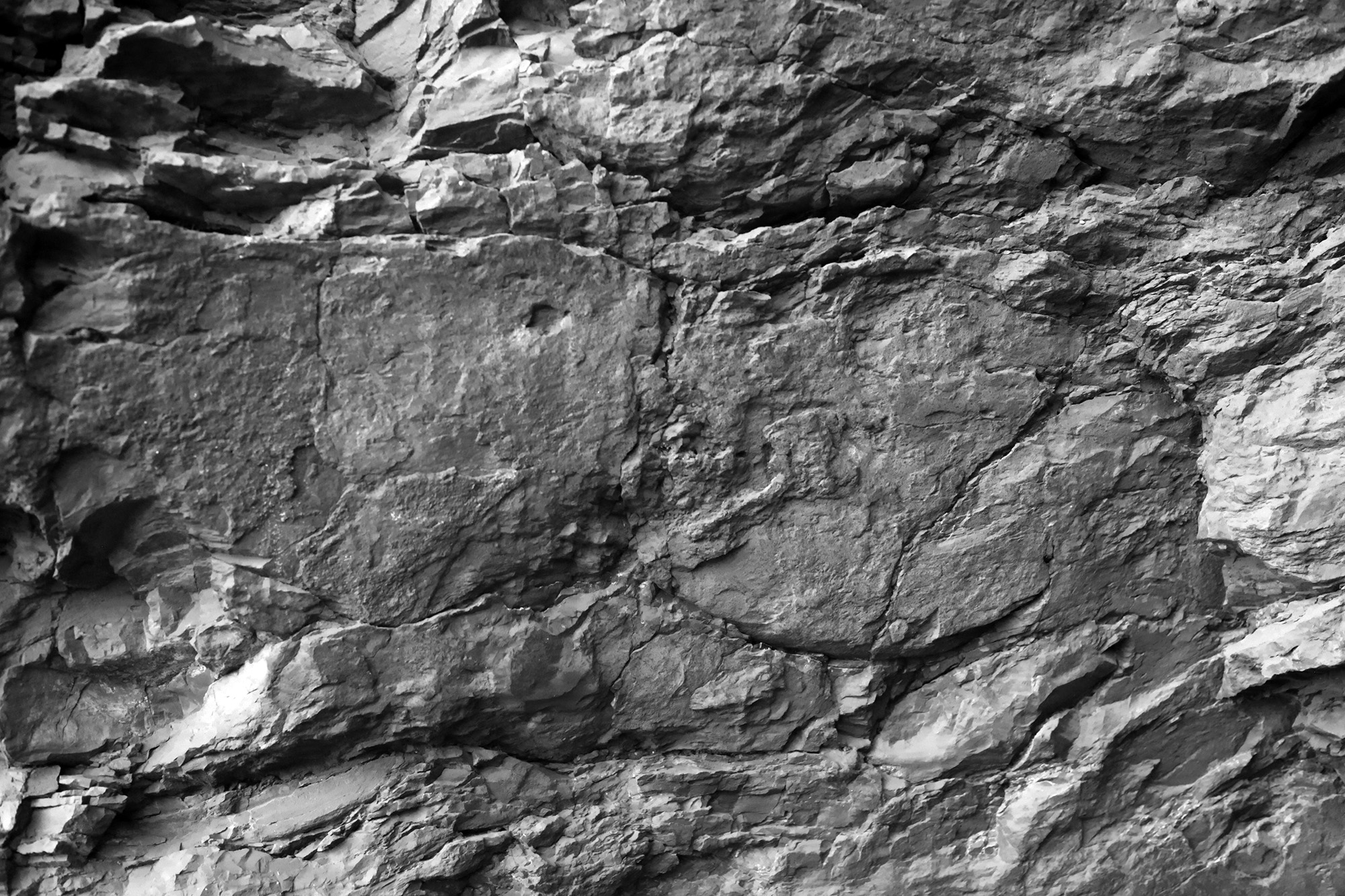
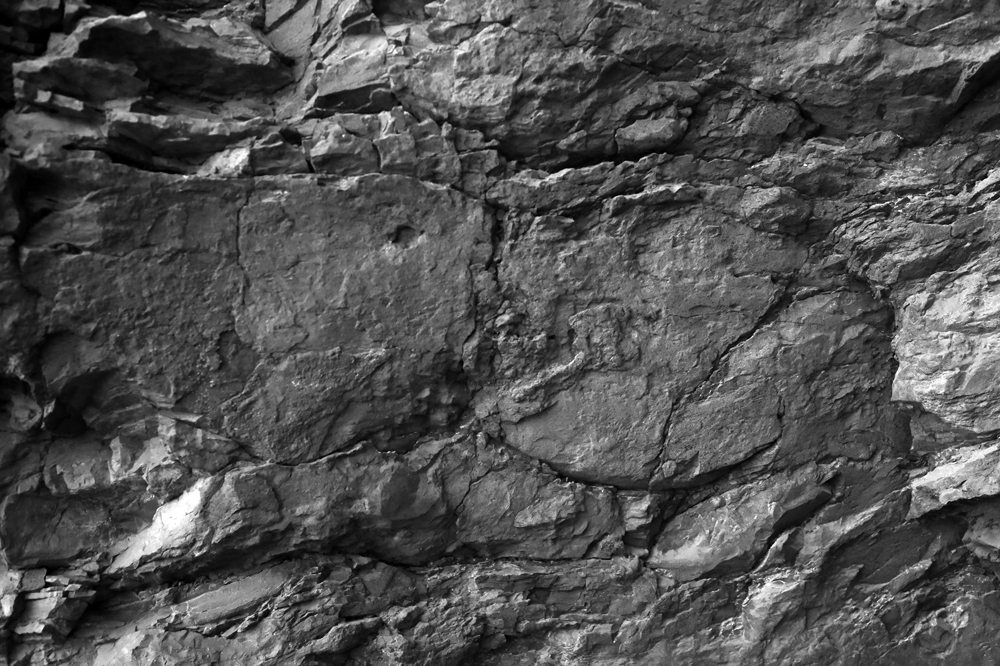
The following are 6 of the photographs (converted to grey scale) from 400nm to 650nm. The 350nm and 690nm photographs are excluded since they received so little energy and were essentially black + noise. The lens was set to manual focus because the method by which the filters were attached to the lens could fall out during the automatic focus action. The ISO on the camera was set to a relatively high 1600, an average aperture of 5.6 and exposure times limited to 2 seconds although in reality the exposure times were mostly under 1/2 second. Since the histogram of each image tended to occupy a limited portion of the available dynamic range, the images have also been level adjusted to spread the histogram over the entire grey scale range.
Vertical "painted" lines are visible in the yellow range while totally absent towards the red end of the spectrum. Enhancing these lines may be achieved by treating the 650nm image as a background/ambient image and subtracting it from the 500nm or 550nm images. The the result of this is shown below. The 11 or 12 vertical lines revealed were not readily observed by other techniques. 
The following is the RGB image from the camera for this second example. Note this was taken at a different time and position and as such the region of interest in the filtered images is larger and to the right of this RGB photograph. 
As in example 1, the following are 6 of the filtered photographs (converted to grey scale) from 400nm to 650nm and histogram equalised.
The composite image below is the 500nm band with the 600nm band subtracted. 

The approach would seem to show promise. While the examples presented are not exciting demonstrations of revealed rock art (due to the nature of the site for this first test), they do show that hitherto hidden or hard to see features can be made visible. Future work
|