|
"TRACE" was an experimental rendering program written in an attempt to
render point fields.....in more interesting ways than with just points.
In many scientific
simulations while points are used for practical computational reasons,
they are intended to be approximations to continuous distributions and
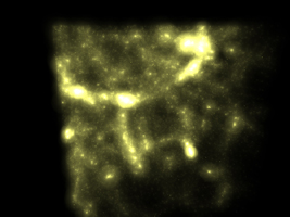
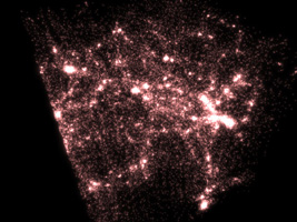
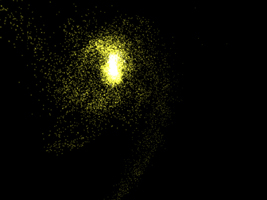
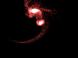
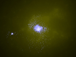
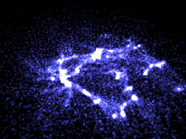
so it makes sense to render them as such. Some initial examples from
this rendering experiment are shown on the right, they are mostly
from astronomy based simulations based upon points that represent
stars, gas, and dark matter.
The overall flow of the program is as follows:
- Initialise internal state, read the data file, set up internal
optimisations, get camera state and other options from either the
command line or default settings file.
- For each pixel in the destination image
create a ray from the camera into the scene. The way this ray
passes through the scene will dictate how the pixel in question is shaded.
- For each point in the scene calculate the closest distance to
the ray. It is this closest distance that acts as an approximation
on how much influence the point has on the ray.
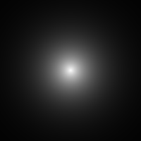
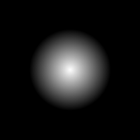
- Evaluate a function of the ray-point distance to determine how
the colour of the ray should change. The different functions are
listed near the end of the document. They are all monotonically
decreasing function of the distance from the origin (data point position).
- Save the resulting image as well as statistical and performance
information.
Data file format
A very simple data format was chosen, it was an ASCII file where each
line represents one point. The first character of the line identifies the
line data type, this could be "#" for a comment or "p" for a point. The
next three items on the line are the x,y,z coordinates of the point.
The next item is the point type (see table below), this is an integer
from 0 upwards. The next item is the spread of the distribution, the
interpretation depends somewhat on the point type. The last three items
on the line are the r,g,b colour of the point. An example data file might be
as follows
# Tests all the datatypes

p -1.4 3  0.5  0  0.1  1 1 1
p -1.0 3  0.5  1  0.1  1 1 1
p -0.6 3  0.5  2  0.1  1 1 1
p -0.2 3  0.5  3  0.1  1 1 1
p  0.2 3  0.5  4  0.1  1 1 1
p  0.6 3  0.5  5  0.1  1 1 1
p  1.0 3  0.5  6  0.1  1 1 1
p  1.4 3  0.5  7  0.1  1 1 1

p -1.4 3 0.0  0  0.075  1 0 0
p -1.0 3 0.0  1  0.075  1 0 0
p -0.6 3 0.0  2  0.075  1 0 0
p -0.2 3 0.0  3  0.075  1 0 0
p  0.2 3 0.0  4  0.075  1 0 0
p  0.6 3 0.0  5  0.075  1 0 0
p  1.0 3 0.0  6  0.075  1 0 0
p  1.4 3 0.0  7  0.075  1 0 0

p -1.4 3 -0.5  0  0.05  1 0 1
p -1.0 3 -0.5  1  0.05  1 0 1
p -0.6 3 -0.5  2  0.05  1 0 1
p -0.2 3 -0.5  3  0.05  1 0 1
p  0.2 3 -0.5  4  0.05  1 0 1
p  0.6 3 -0.5  5  0.05  1 0 1
p  1.0 3 -0.5  6  0.05  1 0 1
p  1.4 3 -0.5  7  0.05  1 0 1
Gives the rendered image below

Optimisation
A brute force approach means that every point is compared and contributes
to every ray. This is obviously wasteful because all point distributions
only affect a local region and if the ray passes further than a points
maximum influence it never contributes or changed the ray. The subset of
points that need to be considered for a ray was reduced by dividing up
the view frustum into an n by n grid and tagging which points can possibly
influence a ray in each grid cell. So when a ray is passing through
a particular cell only those points whose distribution affects that
cell are considered.
|
|


|

