Photomosaics for high resolution image captureWritten by Paul BourkeApril 2014
Translation into Swedish by Eric Karlsson. Introduction
The following will present so called "photomosaics", although in general there is some confusion with the terminology. Photo collages, photo mosaics, image mosaics, gigapixel photographs, panorama photography, etc. Gigapixel and panorama photography assume the camera is rotated about its nodal point, indeed great care is often taken by the photographer to achieve this in order to minimise stitching/blending artefacts arising from parallax errors. Examples of wide angle panoramas are shown in figure 1 and 2. There are a number of reasons for capturing and composing images such as these, the ultra high resolution panoramas stores, in one image, both the detail when zooming in and the context, zooming out. The 360x180 bubble photograph example in figure 2 are often used to give one the sense of a place, everything visible from the camera position is recorded and sometimes this can additionally be at very high resolution. These are often called spherical panoramas or more formally equirectangular projections. 
The resolution of these panoramas is a function of the number of photographs taken, this in turn is often limited by the field of view (FOV) of the lens and for dynamic scenes the time required for a large number of photographs. Each photograph overlaps with its neighbours and feature points between pairs of photographs are used to finally stitch and blend the individual photographs together. 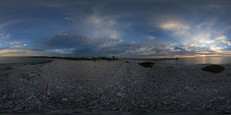 Photomosaics
In what follows the term photomosaic is taken to refer to an image made up of a number of smaller photographs where the camera position varies. Strictly speaking, a photomosaic cannot be perfect except for planar objects. An example of capturing a photomosaic of a planar object is given in figure 3, the image presented is created from a 8x8 grid of photographs taken with a 20MPixels camera and 100mm lens. The resolution of the final image is a function of the field of view of the lens, a narrower FOV means more photographs can be taken. The same feature point detection and stitching that is used for panoramas is deployed in this and subsequent cases. 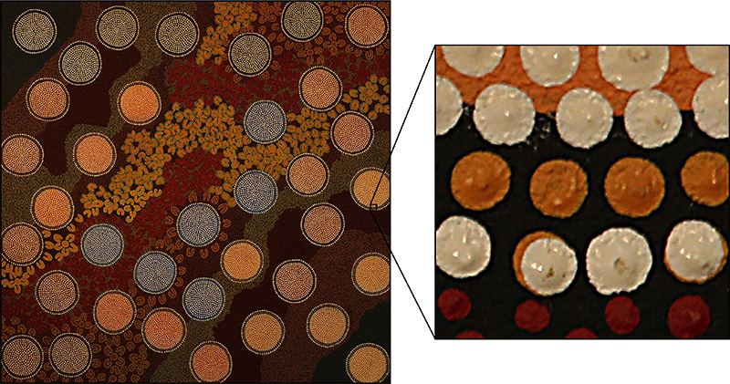 Fundamental limitation
The reason why a perfect stitch as shown in figure 3 cannot be achieved for a scene where there are objects at different depths, consider the situation in figure 4. This shows the side view of two cameras positions with a blue sphere and red cube at different depths in the overlap zone. It is clear that it is not possible to seamlessly blend these two images together. 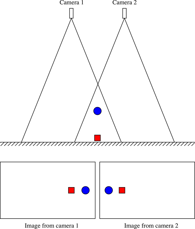
Note that it is possible to blend two images such as the ones illustrated in figure 4 for any particular depth, just not all depths at once. The situation improves for very narrow FOV lenses which increasingly approximates a parallel projection. This is a well known effect for multiple camera video rigs for example, such as the various GoPro rigs and LadyBug series of cameras. While every attempt is made to locate the nodal point of the cameras as close together as possible, this parallax error still exists to some extent and fundamentally limits the stitching quality. Figure 5 shows an example from the LadyBug camera with two blend zones enlarged, the one on the left is at the selected blending distance, the lower right is a closer object with the corresponding blend errors. 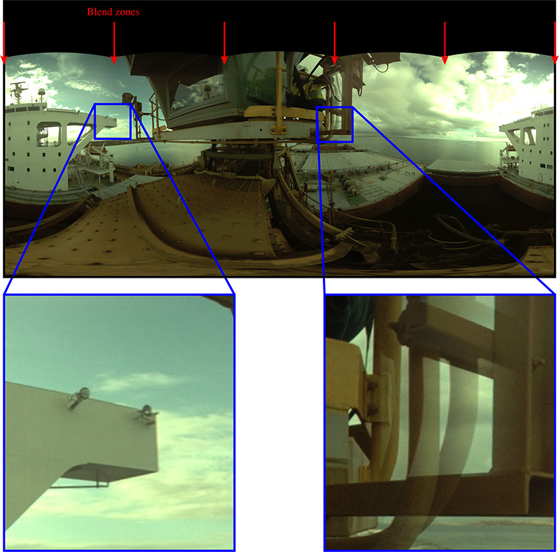
Figure 5. Stitching errors in LadyBug video footage.
All is not lost, in many application there are still benefits in being able to map a large area despite errors in the stitching. The feature point detection and stitching/blending will warp the images in the face of these parallax errors. What one loses is any ability to reliably measure distances and angles, the image warping can be arbitrary in the algorithms attempt to join matched feature points. Examples
In the following examples the camera is moved significantly between photographs, indeed in all cases some attempt was made to move the camera perpendicular to the scene surface. In each, the warping required to match the shared feature points in the photographs is evident. Figure 6 demonstrates the ability of the feature point detection algorithm to be less sensitive to colour information, the photographs here are scans from black and white (greyscale) slides. 
Figure 7 clearly illustrates the discontinuities than can arise from objects at different depths, for example the yellow and black framing which shows discontinuities as the software has preferred to match the deeper decking. 
|