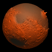
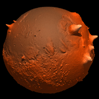
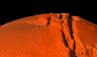
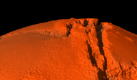
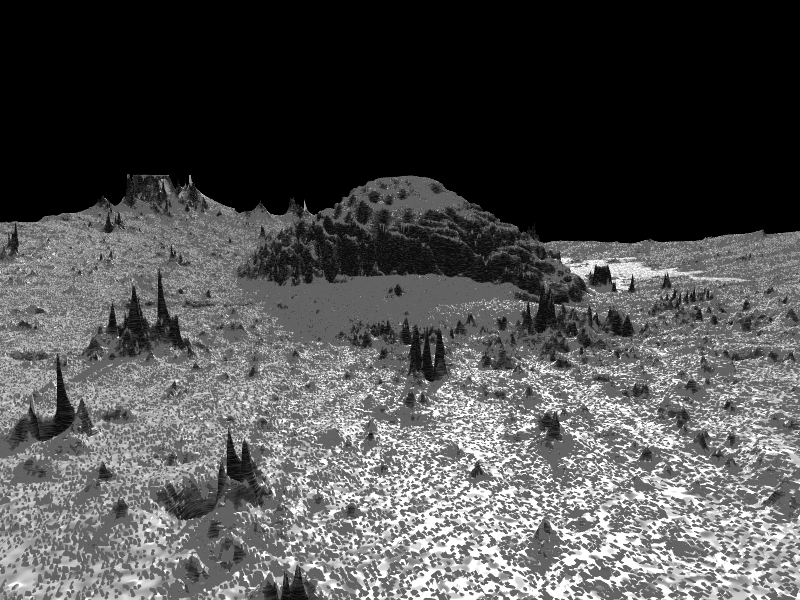
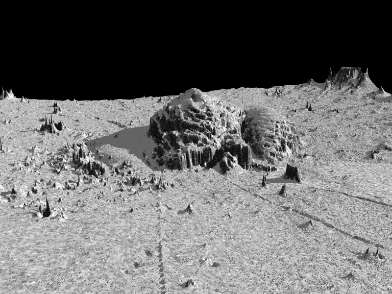
Mars renderings using the 1/8 degree data
Written and rendered by Paul Bourke
October 2000
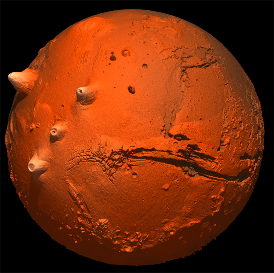
Original rendering
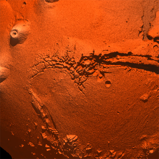
Zoom x 2
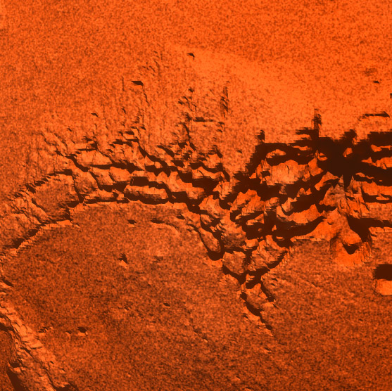
Zoom x 4
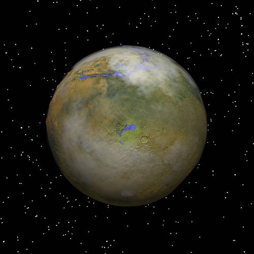
Mars, The Whole Planet
Written by Paul Bourke
July 2000
|
The following renderings were created using PovRay. They are based upon
the 0.5 degree gridded datasets from MOLA
(Mars Orbiter Laser Altimeter).
This is one of the products in the MGS mission
(Mars Global Surveyor).
The mission was launched from Cape Canaveral, Florida, on November 7, 1996
and reached Mars on September 11, 1997.
It is a credit to PovRay that this model, which contains over half a million
triangles renders in less than 5 minutes (600MHz Dec Alpha ev67). In order
to further reduce rendering times for animation sequences, back face
culling was performed before the scene was passed to PovRay for rendering.
This typically reduced the rendering times for each frame to less than
2 minutes.
Input_File_Name=mars.pov
Output_File_Name=mars.tga
Output_to_File=on
Buffer_Output=off
Quality=9
Radiosity=off
Output_File_Type=T
Width=800
Height=600
Antialias=on
Antialias_Threshold=0.1
|
|
|
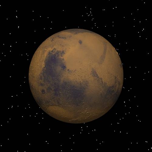
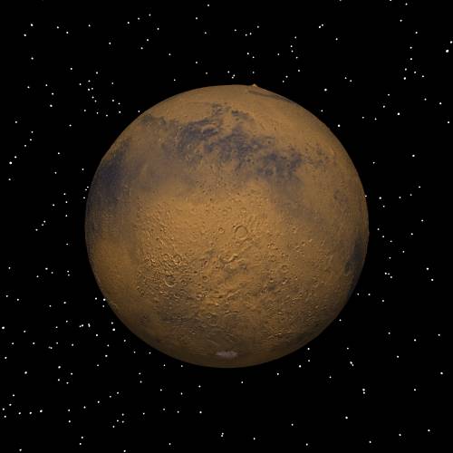
This rendering is with a virtual satellite 10,000 km above the center
of the planet. Given a radius of about 3,500 km, this amounts to
6,500 km above the surface. During the mapping stage of the MGS
mission the real satellite orbited at, on average, 400 km above the surface.
The mapping stage of the mission started in March 1999 and was
expected to last for 1 Mars year, 687 Earth days.
The MOLA data is converted into PovRay triangles, each triangle having
a precomputed colour definition. For technical reasons the triangles
need to be enclosed within a "mesh {}" structure.
mesh {
   triangle {
      <,,>
      <,,>
      <,,>
      texture { Matxxx }
   }
   :
   :
}
|
|
|
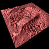
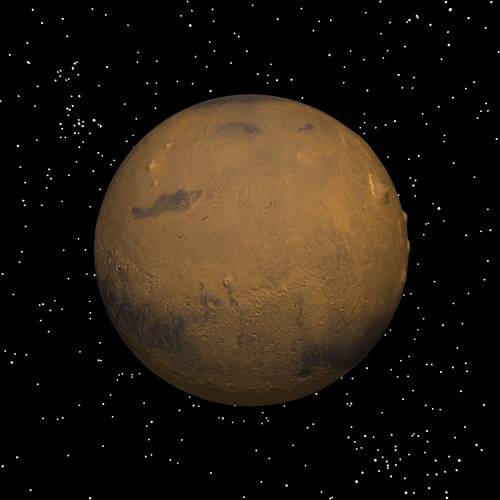
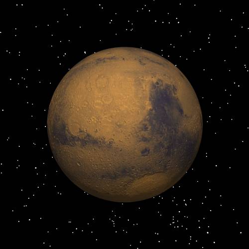
As with most terrain mapping the surface features are exaggerated
in order to make them more noticeable.
The first image on the right has a vertical height scaling of 5.
#declare marsfinish = finish {
   ambient 0.4
   diffuse 1
   specular 0.1
   roughness .1
}

#declare marsnormal = normal {
   bumps 0.5
   scale 5000
}
All the remaining renderings use a height scaling factor of 30.
|
|
|
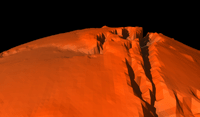
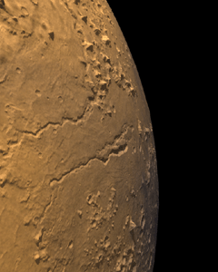
The great rift valley is a deep long crack in the surface, extending almost
5,000 km and 100 km wide in places.
The colour variation in height was created by mapping the following
colour ramp between the lowest and highest elevations.

In total 2000 predefined materials
were created from the colour ramp above, for example the first is:
#declare Matxxx = texture {
   pigment {
      color rgb <0.215686,0.215686,0.176471>
   }
   finish { marsfinish }
   normal { marsnormal }
}
|
|
|
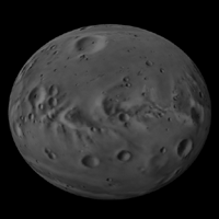
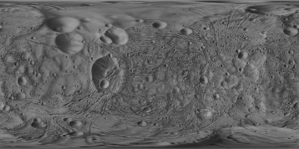
Mars has two moons, phobos and deimos. The orbit of phobos, the larger
of the two moons is 9,378 km which is about the same distance as these
renderings. Deimos is much further away with an orbital radius of
23,459 km.
camera {
   location <10000000,0,0>
   up y
   right 4*x/3
   angle 60
   sky <0,1,0>
   look_at <0,0,0>
}
|
|
|
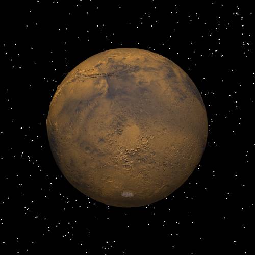
The tallest point on the surface is Olympus Mons which stands about 24
km high but with only 500 km diameter at the base, rising from a smooth plane.
It is a shield volcano but unlike on Earth where plate motion tends
to form strings of volcanoes, on Mars there is no plate motion and
the volcanoes tend to rise up in a single location.
|
|
|
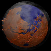
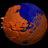
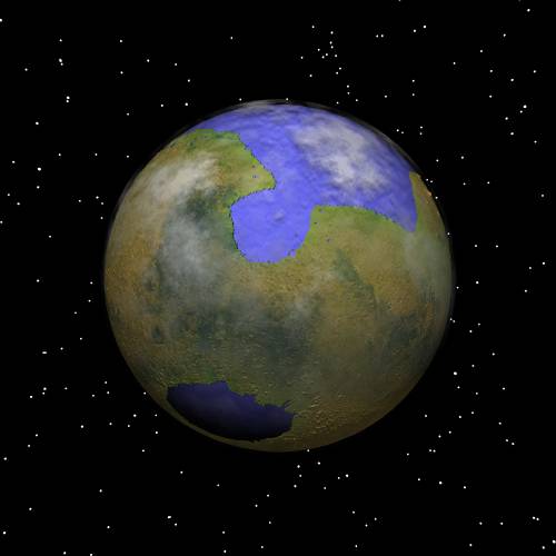
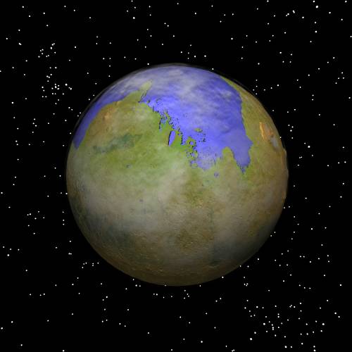
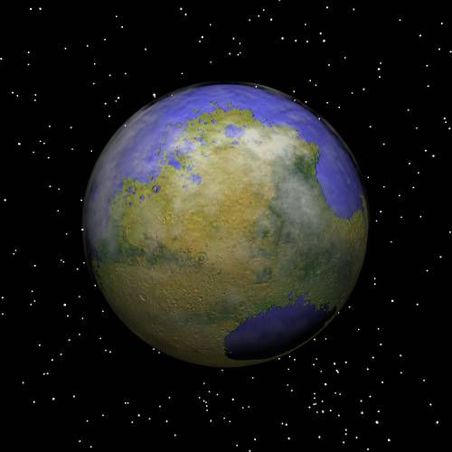
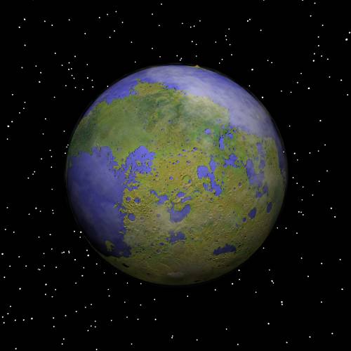
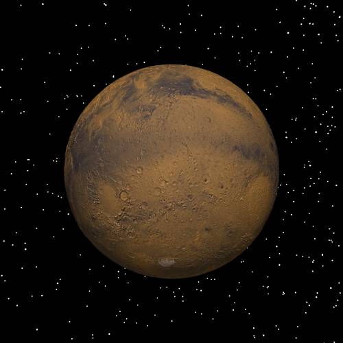
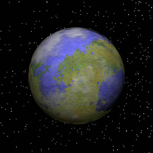
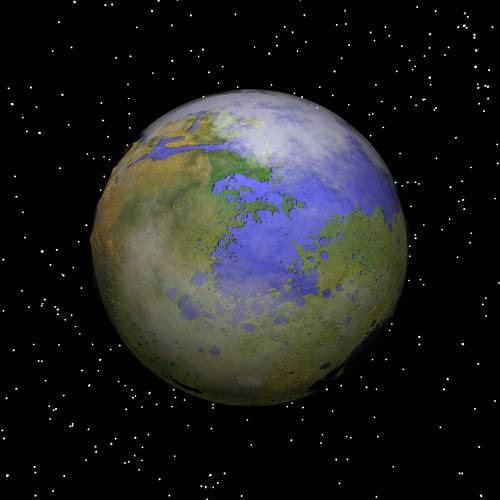
It is a straightforward matter to flood the planet to any arbitrary depth.
#declare seapigment = pigment {
   bozo
   turbulence 1
   octaves 6
   lambda 3
   omega 0.5
   color_map {
      [0.0 color rgbt <0,0,0.7,0> ]
      [1.0 color rgbt <0.5,0.5,1,0> ]
   }
}
sphere {
   <0,0,0>,1
   pigment { seapigment }
   scale 3.35155e+06
}
|
|
|
The first image in this series has an additional cloud cover made up of
carbon dioxide.
sphere { <0,0,0>, 1
   pigment {
      bozo
      phase cloudphase
      turbulence 1
      octaves 6
      lambda 3
      omega 0.5
      color_map {
         [0.0 color rgbt <1,1,1,0.4> ]
         [0.5 color rgbt <1,1,1,1.0> ]
         [1.0 color rgbt <1,1,1,0.4> ]
      }
   }
   scale 3634943.61
   rotate <0,cloudrotate,0>
}
|
|
|
Data resolution
There isn't enough topological detail to get too close to the planet.
At the equator, 0.5 degree sampling results in a resolution of around
30 km.
The image on the right is a view at the equator looking east at a height
of about 100 km above the surface, the facets are clearly visible.
|
|
|
One way of reducing the visual artefacts would be to calculate normals
at the vertices and blend the colours across the facets. While this is
common practice for many rendering applications it gives terrain models
a false impression, landscapes tend to be fractal not smooth. The method
employed here was to use spatial subdivision to generate geometric detail.
The image on the right has had each facet divided into 4 and the introduced
vertices randomly perturbed depending on the local height variation.
|
|
|
The example on the right has each facet subdivided into 16 smaller facets.
The appearance of the facets has been mostly removed, most importantly
the surface still looks like it has detail rather than becoming smooth.
The disadvantage of course is that the geometric detail has increased
significantly, view frustum culling was introduced in order to bring
the polygon count down.
|
|
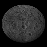
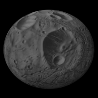
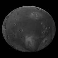
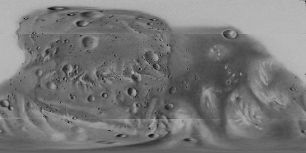
The moons
|
Phobos
light_source { <0,0,-4> White }
light_source { <0,4,0> White }
light_source { <4,0,0> White }

camera {
  location <2.5,0,0>
  look_at <0,0,0>
}

sphere {
   <0,0,0>, 1
   texture {
      pigment {
         image_map { gif "phobos.gif"
            map_type 1
         }
      }
   }
   scale <1,0.820895522,0.686567164>
        rotate <0,clock*360,0>
}
|
|
Deimos
light_source { <0,0,-4> White }
light_source { <0,4,0> White }
light_source { <4,0,0> White }

camera {
  location <2.5,0,0>
  look_at <0,0,0>
}

sphere {
   <0,0,0>, 1
   texture {
      pigment {
         image_map { gif "deimos.gif"
            map_type 1
         }
      }
   }
   scale <1,0.813333333,0.693333333>
        rotate <0,clock*360,0>
}
|
|
In July 2000 the 1/8 degree datasets were released. While this doesn't
particularly alter quality of the renderings given above,
the extra resolution does
permit one to get closer to the surface before artefacts due to
the polygonal faces becomes obvious.
Here are some examples of a 2 and 4 times zoom.
Note that this model has 360*8*180*8*2 or over 8 million triangular
facets. After back face culling this reduced to just over 2 million.
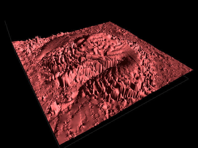
Rendering of the North Pole of Mars
Written by Paul Bourke
September 1999
The data is sourced from the
NASA Planetary Data Systems Geophysics Nodes as part of the
MOLA Mars Orbiter Laser Altimeter project.
An example of the data released by NASA is shown below, it consists
of 1 degree resolution (the 1/4 degree data was not available at the
time of writing).
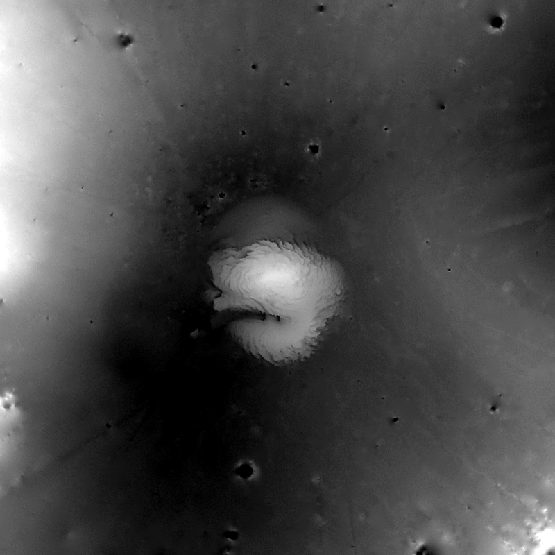
The image is supplied as a 2400x2400 pixel bitmap where each pixel represents
about 2km. The height at each pixel is represented as a 2 byte unsigned
integer, 1 unit representing 1m.
OpenGL
The following renderings are snapshots from an OpenGL version of the
middle third of the dataset centered on the pole region.
With the hardware configuration, this 800x800 grid wa the limit for
interactive flying in OpenGL (Dec Alpha XP1000 with 4D51T OpenGL card)
Note: there is extreme height scaling factor of 2000 in these images!
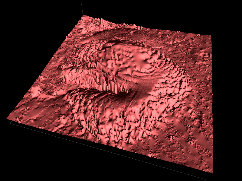
Appeared on the cover of HPCWire magazine on August 17, 2001
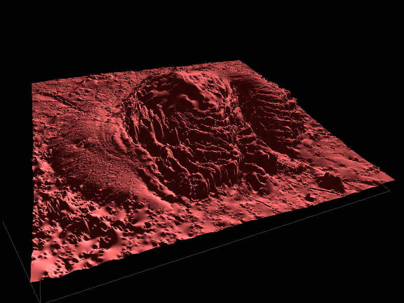
POVRAY
In order to render the entire 2400x2400 grid POVRAY was used primarily
due to it very efficient "height_field" primitive.
In the following renderings the height scale factor is
Source code example for POVRAY
height_field {
   png "mars.png"
   smooth
   pigment {
      color rgb <0.8,0.8,0.8>
   }
   normal {
      bumps 0.5     // The height of the bumps
      scale 0.002   // The spatial scale
   }
   finish {
      ambient rgb <0.2,0.2,0.2>
      phong 1
   }
   translate <-0.5,0.0,-0.5>
   scale <2,0.2,2>
}
There are some artefacts in the data, the following image shows
streaks which illustrate missing or corrupt laser paths.
Online Rendering of Mars
NEWS
This system has now been turned off. It ran for about a month and received
a huge number of hits, unfortunately the cluster it used to do the rendering
has other more pressing activities. Feel free to explore the image gallery
of interesting renderings created while the system was operational.
This experimental interface lets you create your own personal
renderings of the topology of Mars. Simply fill in the form below
and submit it. You will receive an email indicating the eventual
URL of the rendering. Typically your rendering will be ready within
30 minutes but it may take longer depending on the current load
on the farm and the number of other renderings running at the
same time.
The image gallery
has some renderings already created by others.
The renderings are run on the high performance clusters at
Swinburne University and managed by the
Astrophysics and Supercomputing Group. The geometry
is derived from the
MOLA (Mars Orbital Laser Altimeter) 1/32 degree topology dataset.
For more information, suggestions for improvement, and any problems
with this system please contact me (Paul Bourke) by email.
|
|
|
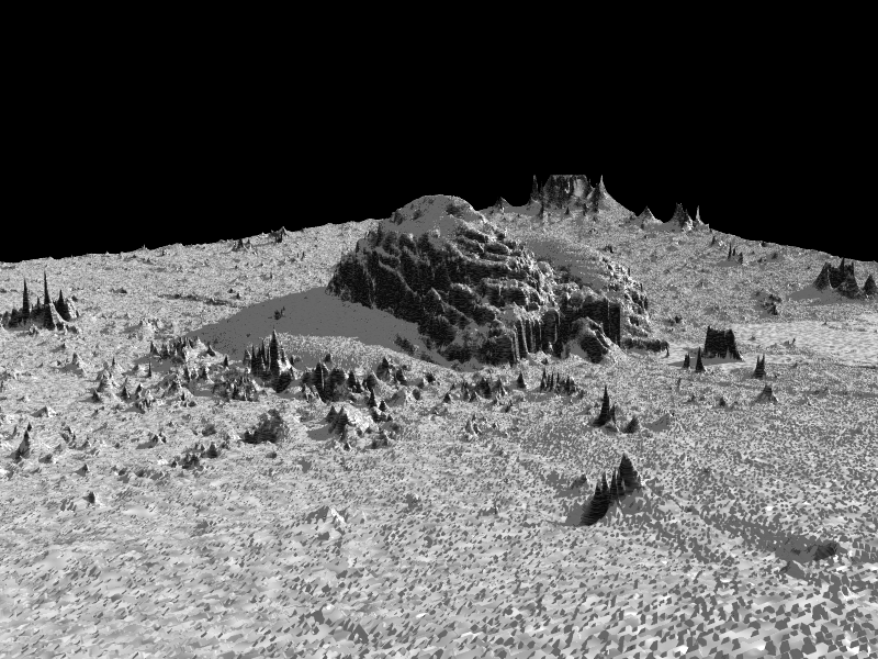
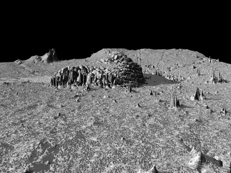
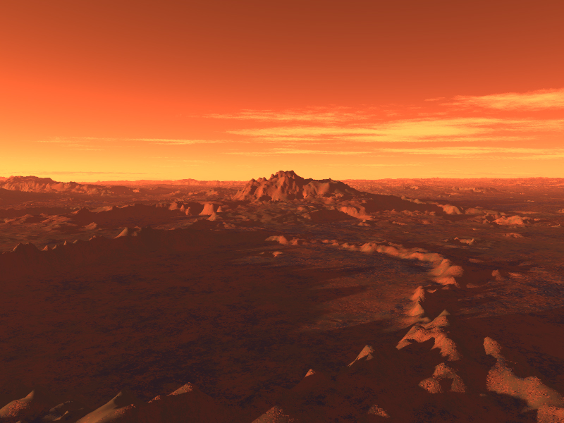
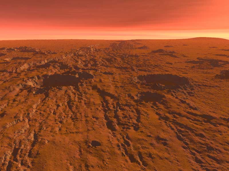
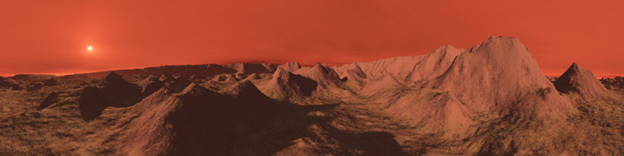
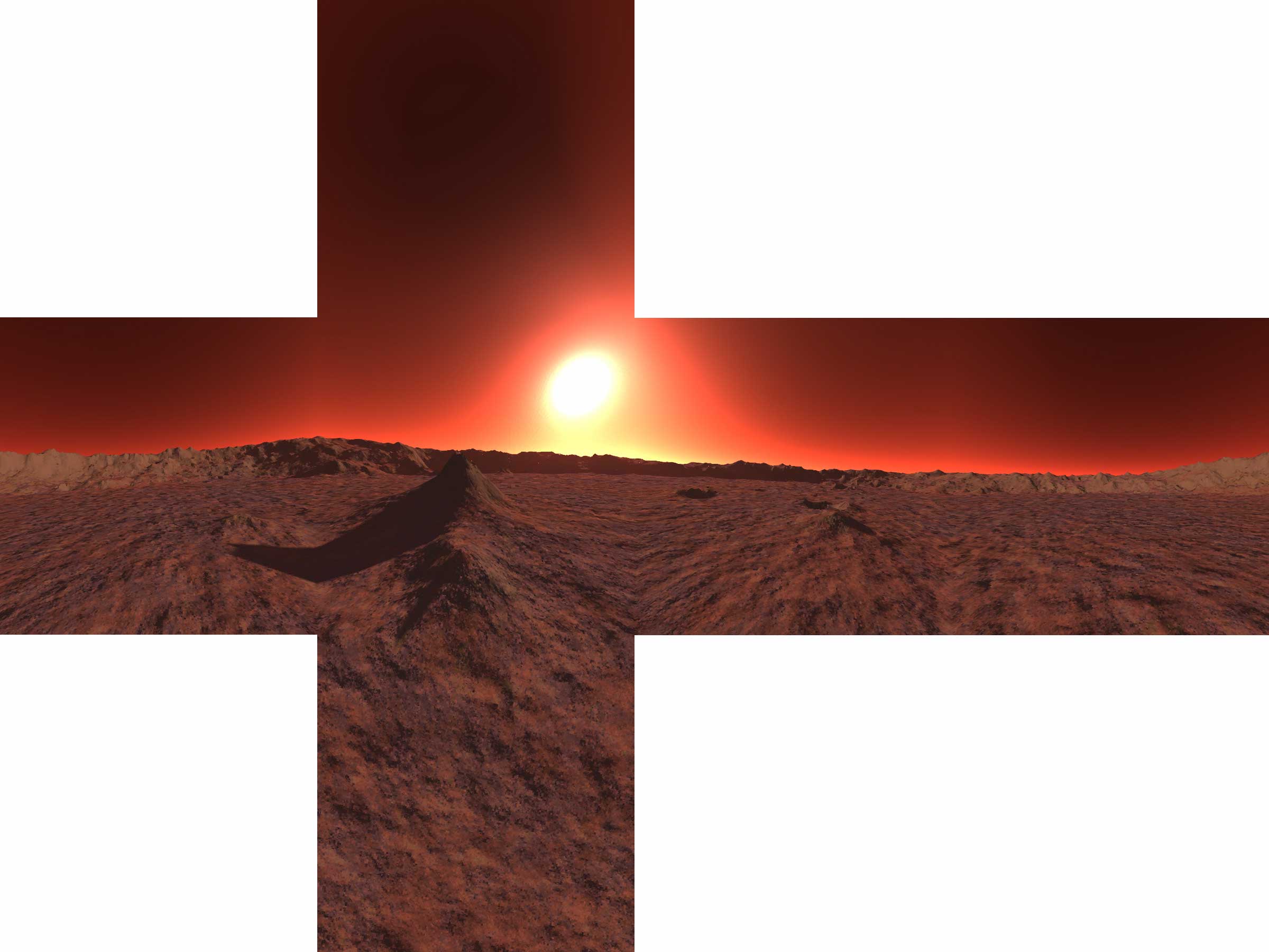
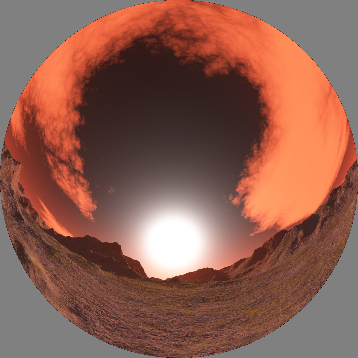
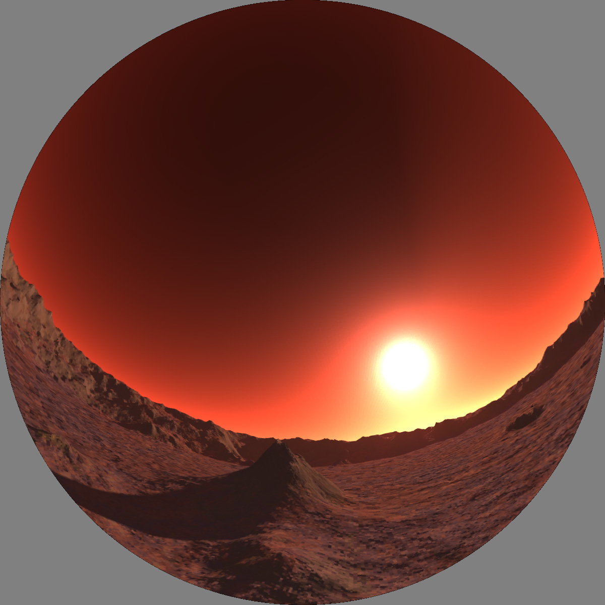
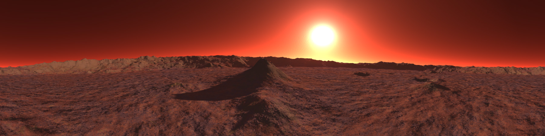
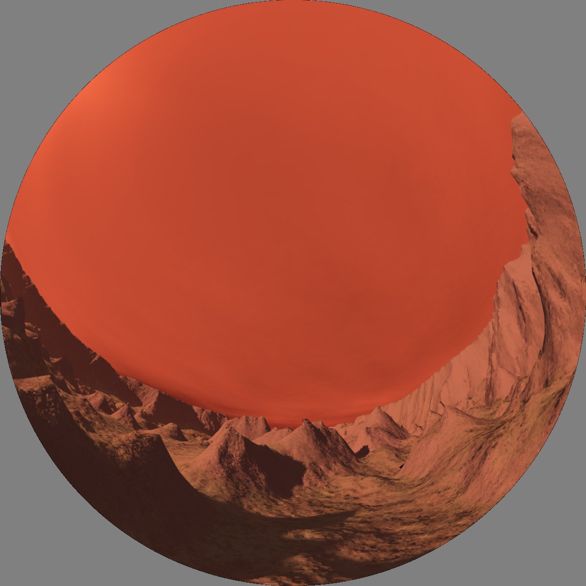
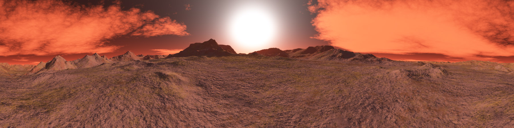
Mars renderings based upon 1/128 degree topology data (MOLA)
Colour tests for terrain and atmosphere
Software: Terragen 0.8.1 (Mac OS-X)
Data: Final MOLA MEGDR maps at 128 pixles per degree
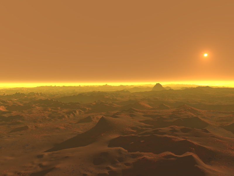
"Random" view from 0o to 44o S
and 180o to 270o N.
Approximately correct Sun size.
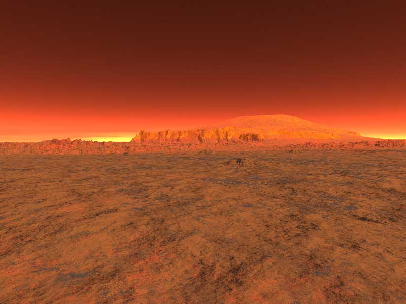
Olympus Mons - the Martian version of Uluru.
"Random" view from 0o to 44o S
and 180o to 270o N
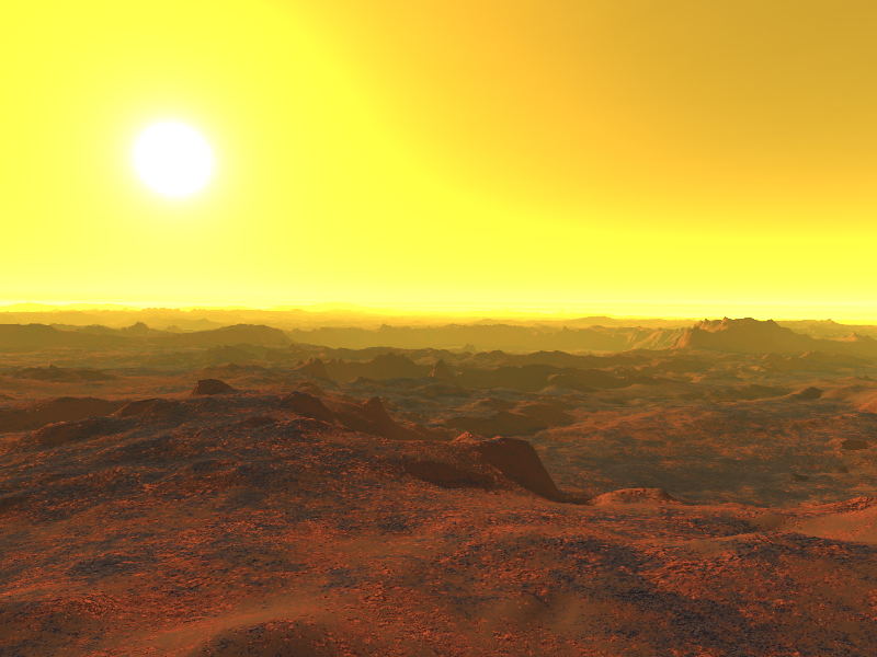
"Random" view from 0o to 44o S
and 180o to 270o N.
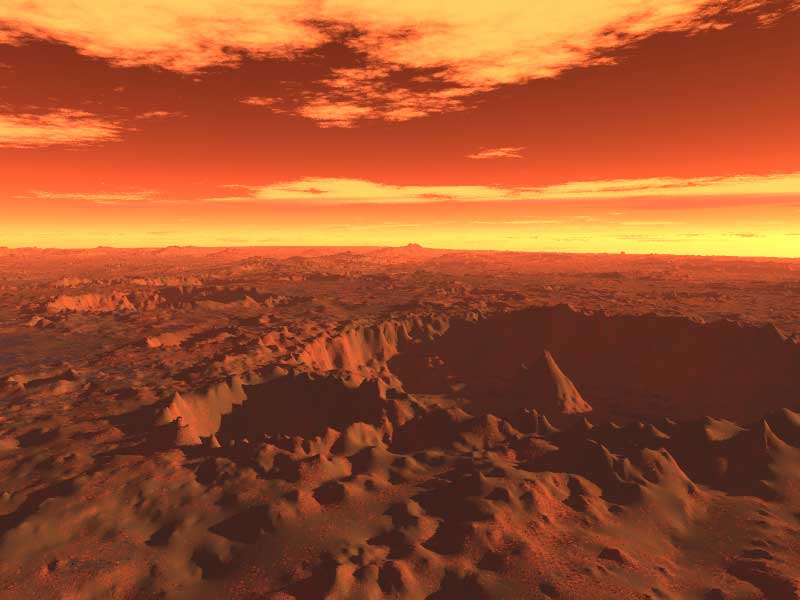
CO2 cloud simulation.
"Random" view from 0o to 44o S
and 180o to 270o N.
Setting Sun.

Olympus Mons
"Random" view from 0o to 44o S
and 180o to 270o N
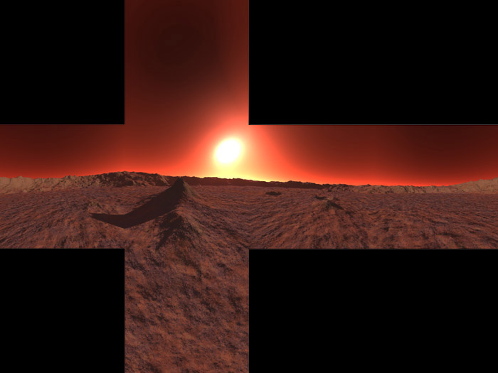
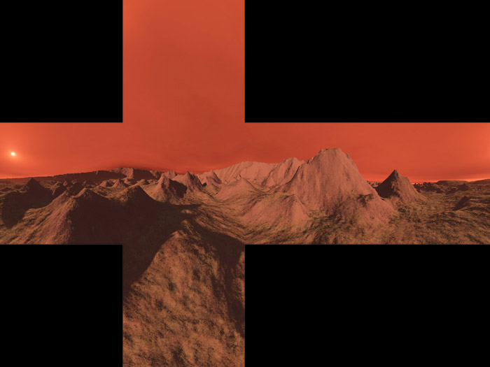
Surround views
Example 1


Example 2

Example 3


|


