|
Introduction
The following outlines a programming project aimed at making full use of
OpenGL based accelerated hardware to render volume datasets at interactive
frame rates (for example, greater than 10 frames per second). It was assumed
that only datasets that fit into main memory would be considered, that is,
disk spooling would not be considered. In addition to "normal" use on a workstation,
another goal was for the software to support stereoscopic projection using either
frame sequential or side-by-side stereo pairs commonly used in passive stereoscopic
projection environments.
Performance
No matter how fast the graphics hardware there will always be volumes of
sufficient resolution to make interactive rates impossible, at the time of writing
and with the graphics cards (nVideo fx2000 and Wildcat 6110)
available this occurred around the 500x500x500 size.
A number of approaches were taken to improve interactivity, they were:
The operator may choose the level of subsampling of the native volume resolution.
This is typically by a factor of 2, 4, or 8. This enables quick exploration,
testing of voxel to colour mappings, and view point considerations. A single
keystroke or menu selection changes the subsampling level.
When the operator is interacting with the model it is subsampled by a factor
of two in all dimensions, typically resulting in a factor of 8 performance
improvement. Interestingly the subsampled data often reveals additional
structure due to the increased transparency because there are half the number of
contributing texture planes.
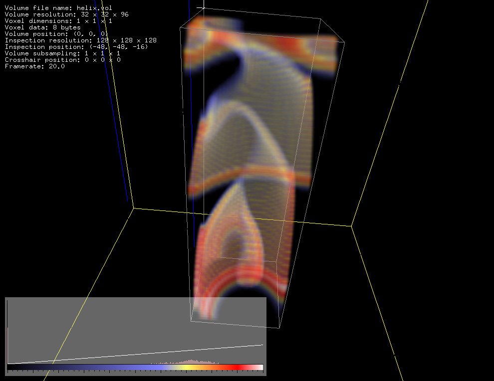
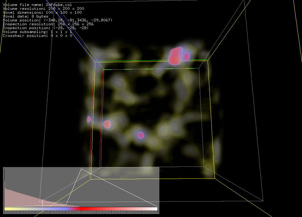
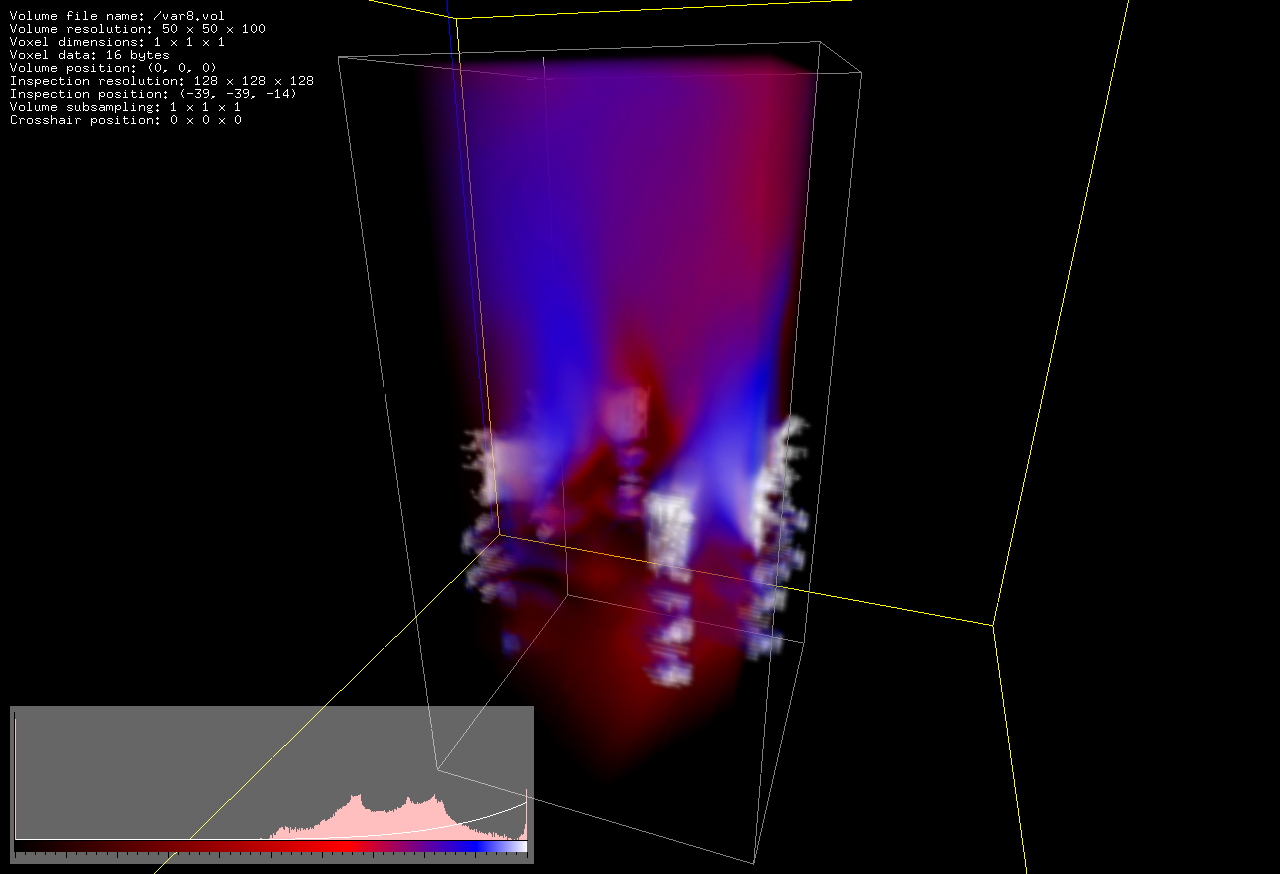
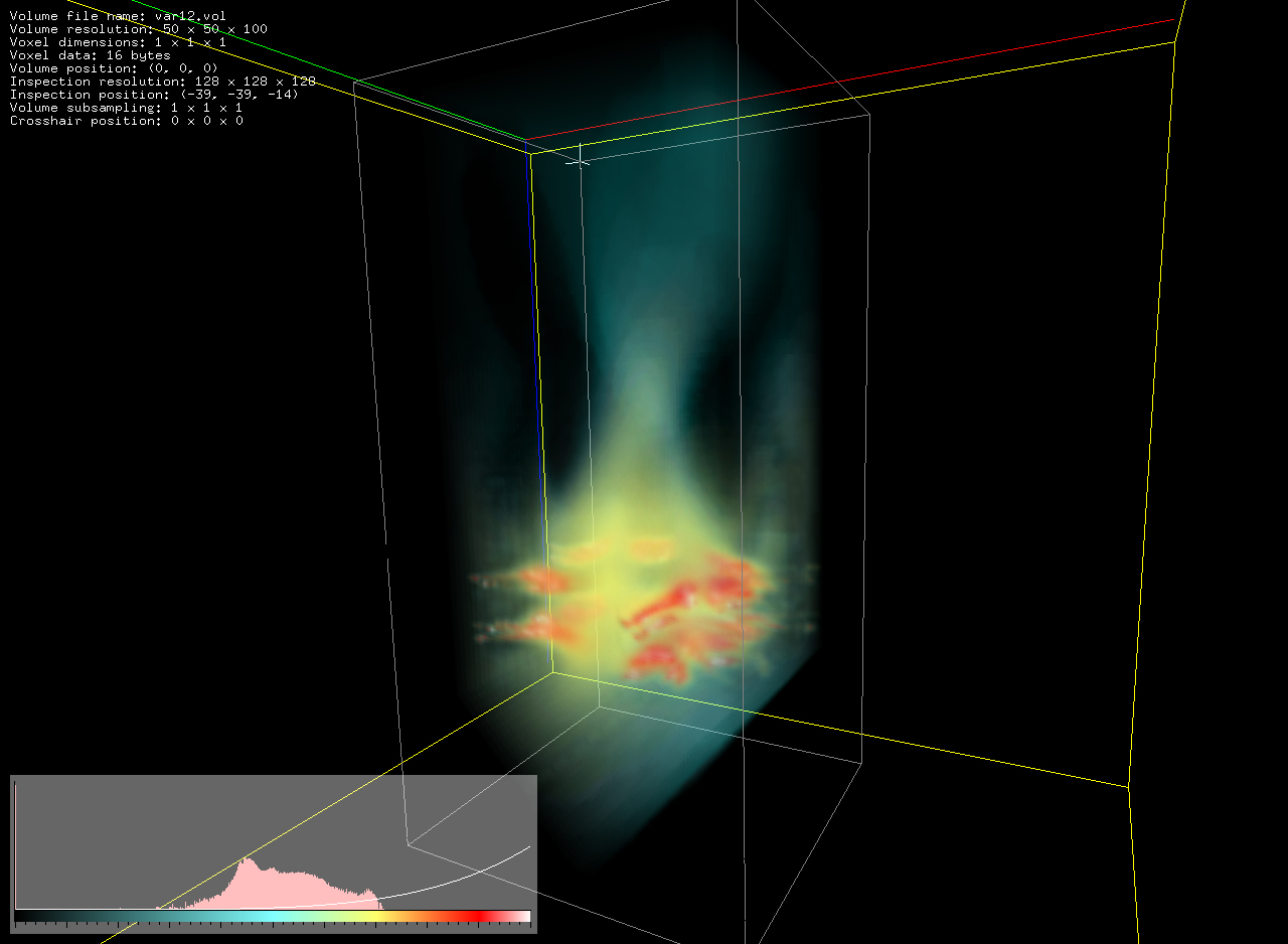
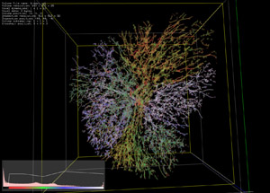
Instead of always looking at the whole volume, a smaller subvolume (shown in
yellow in the images on the right) can be moved around the whole volumetric
dataset (shown in grey on the right). This was initially chosen for performance
reasons but turned out to be a powerful way of exploring large datasets when
one was inside the data volume.
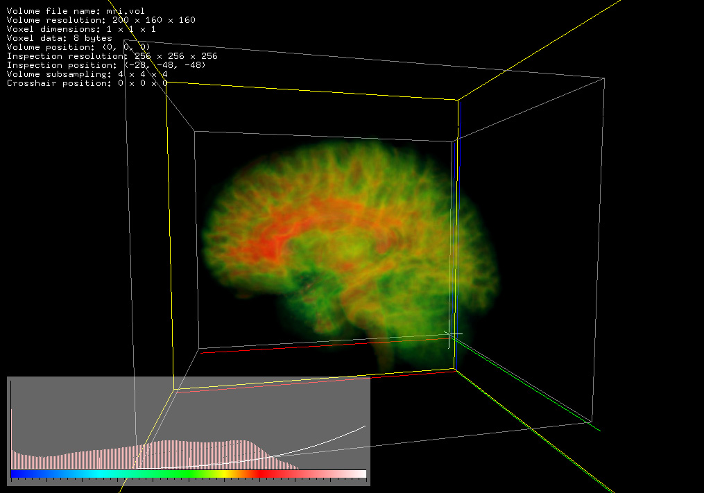
Algorithm
The algorithm uses texture mapped planes implemented in OpenGL.
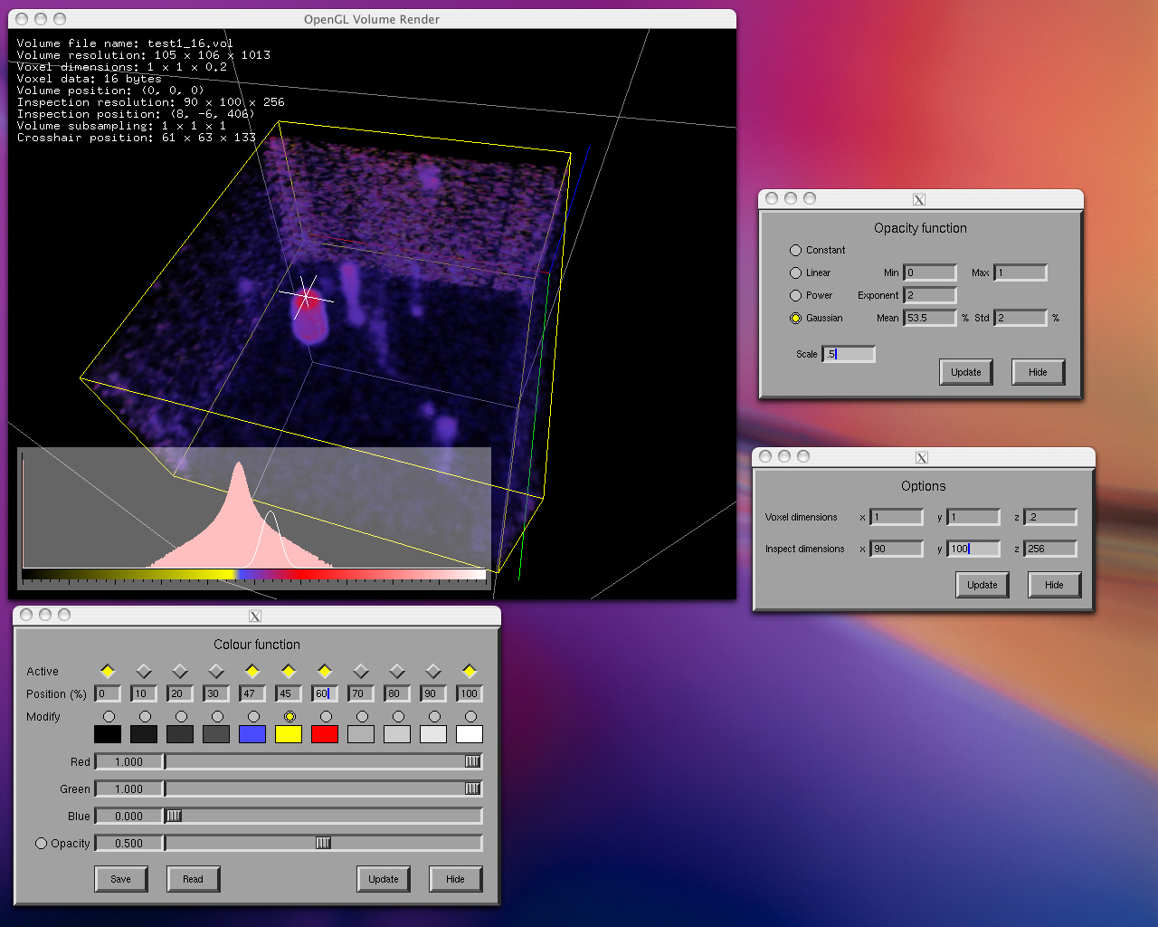
The textures are extracted from the volumetric data after applying a
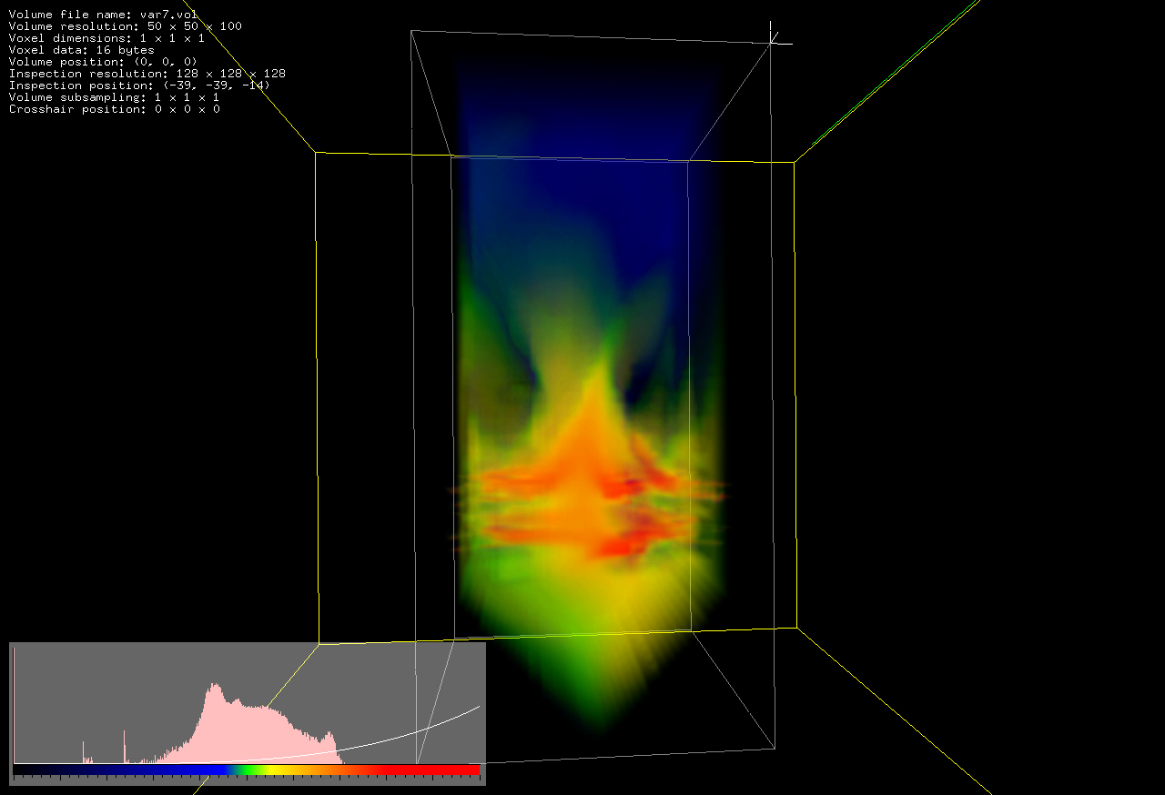
colour/opacity mapping function. This function is shown in the lower left
corner of the images on the right, the pink represents the volumetric data
histogram, the colour map is along the bottom of the histogram and the white
curve indicates the opacity. At the time of writing 8, 16, and 32 bit integer
voxel value datasets are supported as per the
vol file format.
The orientation of the
planes depend on the relative position of the virtual camera. One of three
sets are used, each set is perpendicular to one of the axes of the volumetric
cube. The orientation of the planes
used is the one that is closest to being perpendicular to the
camera view direction, see figure 1 and 2 for examples of two
of the three possible plane orientations (grey lines within yellow subcube).
As the camera passes between the 45 degree edges of the inspection sub volume
the planes are swapped and the new texture set computed. As long as the camera
stays within the current quadrant no reference need be made to the volumetric
data.
The textured planes are additionally
drawn from the back to the front so that the OpenGL blend operators will
work correctly (depth test is disabled).
Figure 1: Orientation of planes
Figure 2: Orientation of planes
Details
Usage: glvol [options] volfile
Options
          -h     this text
          -f     full screen
          -s     active stereo
         -ss     dual screen stereo
          -m s   load map file
          -M s   load marker file
          -r n   initial resolution (1,2,3,4)
         -vx n   initial view volume x size
         -vy n   initial view volume y size
         -vz n   initial view volume z size
          -c s   load camera file
          -a     start in auto rotate mode
          -A n   set tween frames for animation
Key Strokes
  arrow keys     move inspection box
       mouse     rotate/roll camera
           h     move camera to home position
           f     focus camera to current inspection cube
           c     center inspection volume
           w     write current window to a TGA file
           W     write frames to TGA file continuously
         i,k     translate, up/down
         j,l     translate left/right
 x,X,y,Y,z,Z     automatic scanning along axes
         <,>     move camera forward/backward
         +,-     change inspection box size
          f1     toggle decoration display
          f2     toggle texture display
          f3     toggle histogram display
          f4     toggle text information
          f5     toggle camera tracking
          f6     toggle autorotate
          f7     toggle 3d cursor
     1,2,3,4     set supsampling level to 1,2,4,8
           q     quit
| |
|
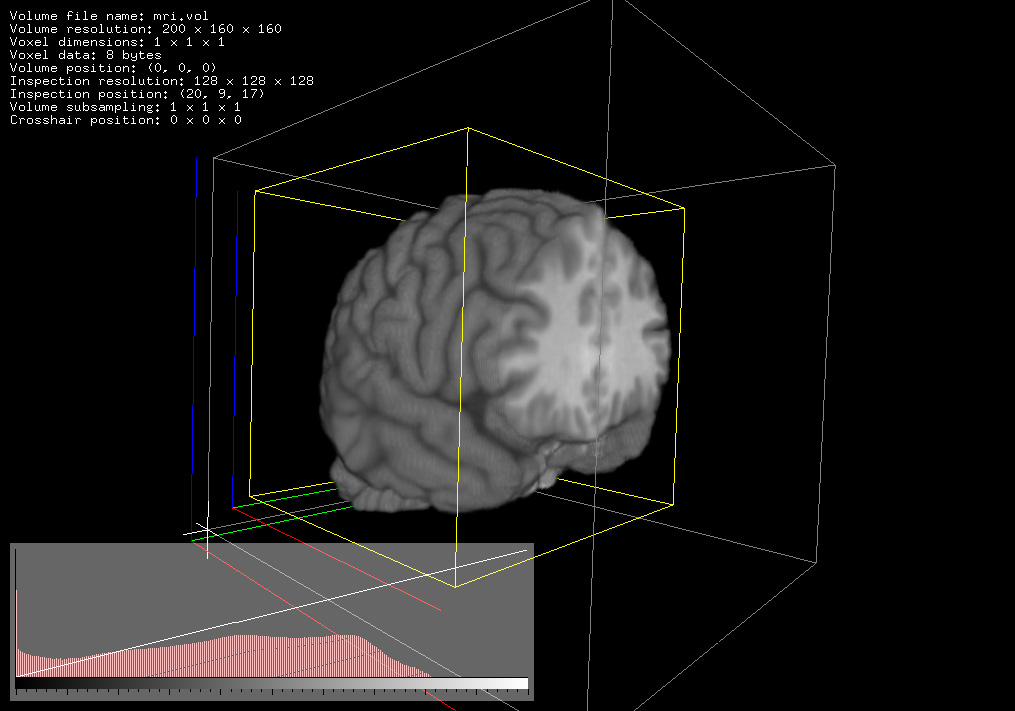
MRI data
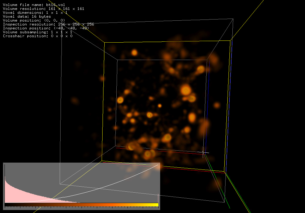
Volumetric data courtesy of Brent Tully
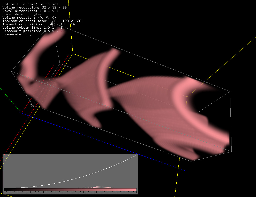
Helix waves
2dF subvolume

Screen dump
Ducts
|