Miscellaneous functions

Zeta function

The Zeta function (sometimes called the Riemann Zeta Function) was defined by Euler as

Where z is a complex number with the real part greater than 1.

An alternating sign version is defined as

Where the real part of z must be greater than 0. This allows the zeta function to be defined for real values of z greater than 0 but not 1 as follows.

There are some special values of the zeta function that are known, for example zeta(2) = pi² / 6, zeta(4) = pi⁴ / 90, zeta(6) = pi⁶ / 945. For the alternating zeta function zeta_a(2) = pi² / 12, zeta_a(4) = 7 pi⁴ / 720.

A well known (and unproven) hypothesis is called the Reimann Hypothesis is that all values of z for which zeta(z) = 0 are of the form 1/2 * i y. That is, a complex number with real part of 1/2.

Alpha Function

SINC function

The so called "sinc" function turns up in many application areas, perhaps most often in signal processing and Fourier analysis as it is the form of the Fourier transform of a rectangular pulse. The usual definition is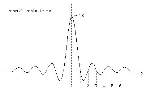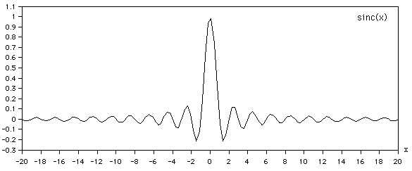

Generating the function in software is straightforward noting the special case near the origin. Since sin(x) is very close to linear as x -> 0, there are no numerical problems using a low order polynomial expansion for sin(x) in this region.

Factorial and the Gamma Function

The factorial of an integer n is normally written as n! and defined as

The factorial is a special case of the more general Gamma function which can be applied to any real (or complex) number. The Gamma function is defined as

When the Gamma function is applied to the positive integers its relationship to factorials is as follows

Note:

• 

• The gamma function of 0.5 is of pi^1/2

• Gamma(3/2) = 0.5 pi^1/2

Gamma(x+1) = 1 - 0.577191652 x + 0.988205891 x² - 0.897056937 x³ + 0.918206857 x⁴ - 0.756704078 x⁵ + 0.482199394 x⁶ - 0.193527818 x⁷ + 0.035868343 x⁸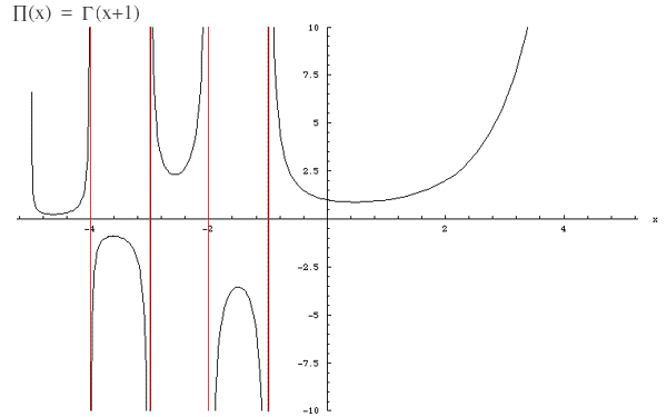

/*
   Natural log of the gamma function (xx > 0)
   Derived from "Numerical Receipes in C"
*/
double LnGamma(double xx)
{
   int j;
   double x,y,tmp,ser;
   double cof[6] = {
      76.18009172947146,    -86.50532032941677,
      24.01409824083091,    -1.231739572450155,
      0.1208650973866179e-2,-0.5395239384953e-5
   };

   y = x = xx;
   tmp = x + 5.5 - (x + 0.5) * log(x + 5.5);
   ser = 1.000000000190015;
   for (j=0;j<=5;j++)
      ser += (cof[j] / ++y);
   return(log(2.5066282746310005 * ser / x) - tmp);
}

Handbook of Mathematical Functions
Abramowitz, M., and Stegan, I.A.
9th Edition, Chapter 6, pp 255.

Gabor Function

The Gabor function is the name given to a Gaussian weighted sinusoid. In higher dimensions the sinusoid only varies in one dimension while the Gaussian envelop applies in all dimensions. The function is named after Dennis Gabor who used this function in the 1940s and later J Daugman who proposed the function to describe the spatial response of cells in visual stimuli experiments.

The center of the function is at "m", the width is given by the standard deviation "s" of the Gaussian, the number of cycles within the envelop is T.

The function for various values of the cosine period "T".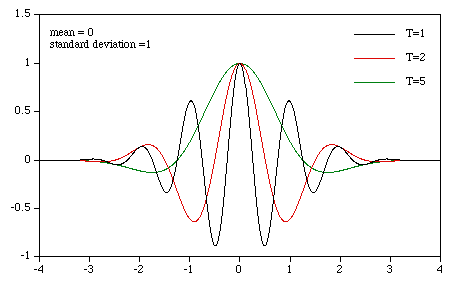

2 Dimensions The equation in 2D is as follows

The parameters have a similar meaning in 2 dimensions except that now there are two parameters for the center (m_x, m_y) and standard deviation (s_x, s_y).

3D perspective surface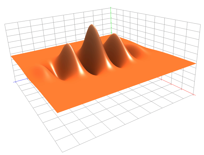

Note

• On occasion the periodic term contains a phase shift "p", for example, something of the form
  cos(2 pi (x - m) / T + p)
  
• In 2D it is possible to include an angle for the primary axis but it is more common to simply rotate the function above which is aligned along the x axis.

Sigmoid Function

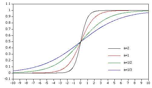
This function arises in many dynamical systems because it is the solution to a first order differential equation

This equation describes simple exponential growth dynamics with a linear limiting control, such systems are often called logistic growth or Verhulst growth. The solution is

Gompertz Function

The Gompertz equation arises from models of self-limited growth where the rate decreases exponentially with time, for example, as the solution to the first order differential equation

The solution is of the form

where a and k are greater than 0.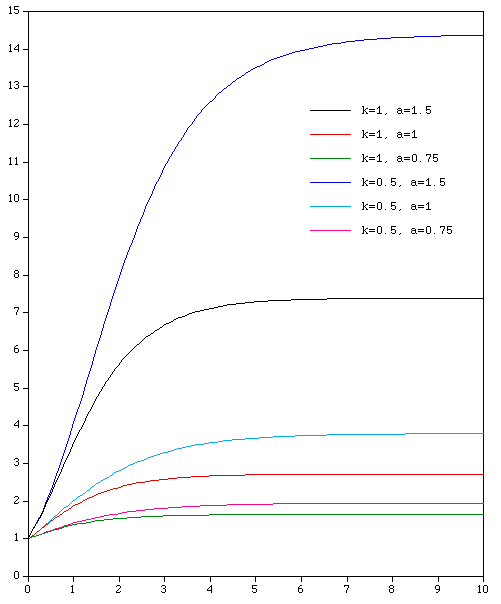

Biexponential Function

The biexponential function is defined as follows.

Where a,b,t greater than or equal to 0, a is not equal to b.

When a = b the function is f(t) = a² t e^{- a t}

The form of the function for one value of a and a number of different values of b is shown below.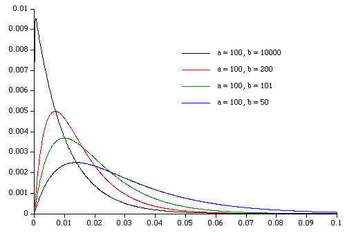

Notes

• The constant ab / (a - b) serves to normalise the area under the function to unity.

• The maximum occurs at t = (b - a)^-1 log_e(b / a)

• For a = b the maximum occurs at 1 / a

• If b is very much larger than a then the function approximates an exponential.

There is a computationally nice result when using a biexponential in a convolution, say f_t = biexp_t * g_t Normally one would need to remember the last N terms of g_t where N is determined by how far along the biexponential one wished to perform the convolution. It can be shown however that the convolution can be performed with a minimum of storage as

Where

and

Miscellaneous Series and Sequences

Definitions
Sequence - An ordered list of numbers determined by some rule.
Series - Sum of the terms in a sequence.

Arithmetic series

   a + (a+d) + (a+2d) + (a+3d) + ..... + (a+(n-1)d) = n (2 a + (n - 1) d) / 2

   a + ar + ar2 + ar3 + ..... + arn-1 = a (1 - rn) / (1 - r), for r not equal to 1

   1 + x + x2/2! + x3/3! + ..... = ex

   x + x2/2 + x3/3 - x4/4 + ..... = loge(1 + x)

   (1 + x)n = 1 + nx + n(n-1)x2/2! + n(n-1)(n-2)x3/3! + .....

Sine and Cosine

   x - x3/3! + x5/5! - x7/7! + ... = sin(x)
   1 - x2/2! + x4/4! - x6/6! + ... = cos(x) 

   1 + 1/2 + 1/3 + 1/4 + 1/5 + 1/6 + 1/7 + . . . . + 1/n + . . . = infinity

Prime Harmonic Series

   1/2 + 1/3 + 1/5 + 1/7 + 1/11 + 1/13 + 1/17 + 1/19 + 1/23 + . . . .

   1 + 2 + 3 + 4 + .... + n = n (n + 1) / 2
   12 + 22 + 32 + 42 + ..... + n2 = n (n + 1) (2 n + 1) / 6
   13 + 23 + 33 + 43 + ..... + n3 = n2 (n + 1)2 / 4 

   F[n] = F[n-1] + F[n-2]
   for integers F[0] and F[1]
   1, 1, 2, 3, 5, 8, 13, 21, 34, 55, 89, . . .

   Q[n] = Q[n-Q[n-1]] + Q[n-Q[n-2]] 
   Q[0] = 1, Q[1] = 1
   1, 1, 2, 3, 3, 4, 5, 5, 6, 6, 6, 8, 8, 8, 10, 9, 10, 11, 11, 12, . . .

Pascals triangle

               1
             1   1
           1   2   1
         1   3   3   1
       1   4   6   4   1
     1   5   10  10  5   1
   1   6   15  20  15  6   1
   :   :   :   :   :   :   :

Perfect number sequence
Numbers in this sequence are those that are equal the sum of every smaller integer that divides it without remainder.
eg: 6 = 1 + 2 + 3 and can be divided perfectly by 1, 2, and 3.
eg: 28 = 1 + 2 + 4 + 7 + 14

   6, 28, 496, 8128, 33550336, 8589869056, 137438691328, 
2305843008139952128, ...

These number all satisfy 2^p-1 (2^p-1) where 2^p-1 is prime, called a Mersenne prime. Note: p will also be prime.

Trigonometric Identities

sin(a +/- b) = sin(a) cos(b) +/- cos(a) sin(b)

cos(a +/- b) = cos(a) cos(b) -/+ sin(a) sin(b)

2 sin(a) cos(b) = sin(a + b) + sin(a - b)

2 cos(a) cos(b) = cos(a + b) + cos(a - b)

2 sin(a) sin(b) = cos(a - b) - cos(a + b)

                tan(a) +/- tan(b) 
tan(a +/- b) = -------------------
               1 -/+ tan(a) tan(b)

sin(2 a) = 2 sin(a) cos(a)

cos(2 a) = 1 - 2 sin(a) sin(a) = cos(a) cos(a) - sin(a) sin(a) = 2 cos(a) cos(a) - 1

               2 tan(a)
tan(2 a) = -----------------
           1 - tan(a) tan(a)
     
                        a + b      a - b
sin(a) + sin(b) = 2 sin(-----) cos(-----)
                          2          2

                        a + b      a - b
sin(a) - sin(b) = 2 cos(-----) sin(-----)
                          2          2

                        a + b      a - b
cos(a) + cos(b) = 2 cos(-----) cos(-----)
                          2          2

                        a + b      a - b
sin(a) - sin(b) = 2 sin(-----) sin(-----)
                          2          2

sin(a) sin(a) + cos(a) cos(a) = 1

tan(a) tan(a) = sec(a) sec(a) - 1

Substituting t = tan(a/2) then
                 2 t                 1 - t t                 2 t
      sin(a) = -------      cos(a) = -------      tan(a) = -------
               1 + t t               1 + t t               1 - t t

Definitions
      sec(a) = 1 / cos(a)         cosec(a) = 1 / sin(a)
      tan(a) = sin(a) / cos(a)    cot(a) = 1 / tan(a)

eia = cos(a) + i sin(a)    where i = sqrt(-1)

Gaussian (Normal) Distribution

The Normal or Gaussian distribution plays a central role in statistics and has been found to be a very good model for many continuous distributions that occur in real situations. The Gaussian function with mean (m) and standard deviation (s) is defined as follows:

The function is symmetric about the mean, it gains its maximum value at the mean, the minimum value is at plus and minus infinity. The distribution is often referred to as "bell shaped", it has the following typical form.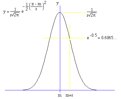

At one standard deviation from the mean the function has dropped to about 2 thirds of its maximum value, at two standard deviations it has fallen to about a seventh of its maximum value.

The area under the function one standard deviation from the mean is about 0.682. Two standard deviations it is 0.9545, and three standard deviations it is 0.9973. The total area under the curve is 1, as the standard deviation is increased the curve broadens, for example the following shows the distribution for a number of values of s.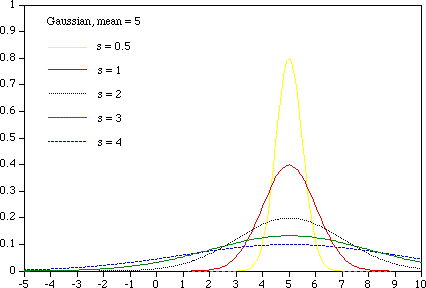

2D Gaussian

For a radially symmetric 2D Gaussian centered at the origin (mean = 0)

The total volume under a 2D Gaussian is 2 pi s_x s_y.

Poisson Distribution

The probability distribution function for a Poisson process is defined as

Lambda is often a rate per unit time, distance, or area.

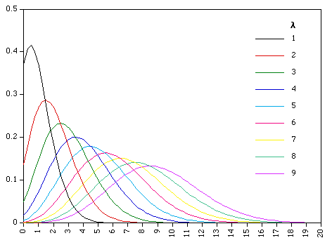
It satisfies the main requirement for a probability density function, namely that

For the proof of this consider the Maclaurin infinite series expansion

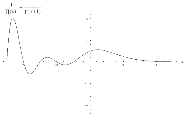
A binomial process with large n (number of samples or events) and small p (probability of an event) but such that the mean np is constant tends to Poisson. lambda = np.

Details - Factorial of a continuous variable

y! for a continuous variable is defined using the gamma function, namely Gamma(y+1).

A snippet of C code based on the algorithm in "Numerical Recipes in C" is given below for computing the natural logarithm of Gamma(y) for y > 0.

double LnGamma(double xx)
{
   int j;
   double x,y,tmp,ser;
   double cof[6] = {
      76.18009172947146,    -86.50532032941677,
      24.01409824083091,    -1.231739572450155,
      0.1208650973866179e-2,-0.5395239384953e-5
   };

   y = x = xx;
   tmp = x + 5.5 - (x + 0.5) * log(x + 5.5);
   ser = 1.000000000190015;
   for (j=0;j<=5;j++)
      ser += (cof[j] / ++y);
   return(log(2.5066282746310005 * ser / x) - tmp);
}

Gamma Distribution

The probability density function for a gamma distribution is given in most general terms as

where a and b are both greater than 0. The "standard" gamma function is often quoted as having B = 1. The gamma distribution formula above requires the evaluation of the gamma function defined as

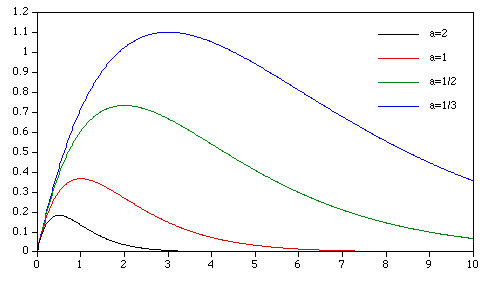
Examples of the gamma distribution for a range of values of a but a fixed value of B=1 are shown below. If a <= 1 then the distribution is always decreasing.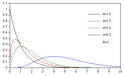

The following shows the gamma distribution with a fixed value of a=2 and various values of B. B acts mostly to stretch the distribution in the x direction.

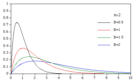
The mean of a gamma distribution is the product of a and B. The variance is the product of a and the square of B.

The exponential distribution is a special case of the gamma distribution where a=1 and B = 1/lambda.

Exponential Distribution

The probability distribution function of an exponential distribution is given by

The mean is 1/lambda, the variance is 1/lambda² Integrating the above gives the cumulative distribution

Some examples of the exponential distribution for various values of lambda are shown below: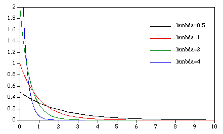

To generate an exponential distribution with a mean "m" from a uniform distribution "u" on (0,1) use -m ln(u).

Rayleigh Distribution

The probability distribution of a narrow band noise process n(t) was formulated by Rice in papers published in the Bell Laboratories Journal, 1944 and 1945. It can be derived by considering a complex phaser

where r(t) is the magnitude or envelope and phi(t) is the phase. This can also be written in terms of its real and imaginary parts (in-phase and quadrature components) as

If both random processes x(t) and y(t) are Gaussian distributed with the same variance and zero mean then the probability density functions P(x) and P(y) are given by

Assuming x and y are statistically independent then

Transforming differential areas using

gives the joint probability density function as

Since this is independent of phase the random variables r and phi are statistically independent and therefore

Then

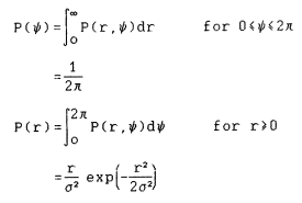
This is normally called the Rayleigh Distribution. See figure A.1 for plots of this distribution for various values of the variance.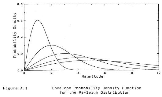

• The random variable phi is uniformly distributed between 0 and 2 pi.
  
• The maximum of P(r) occurs when r = sigma, and
  

• Compared to the Gaussian Distribution P(r) is zero for negative r.

Rice Distribution

The probability distribution of a sinusoid plus narrow band noise is called the Rice Distribution. The expression for a cosinusoid of amplitude A and noise process, as for the Rayleigh distribution, can be written as

The Rician probability density function is derived as for the Rayleigh distribution by considering the in-phase and quadrature components. The joint probability density function in this case is

where now r and phi are no longer statistically independent variables. The envelope distribution P(r) is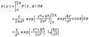

where I_o is the zero order modified Bessel function of the first kind (Abramowitz 1970) given by

The phase distribution is

where erf(x) is the error function (Abramowitz 1970) defined as

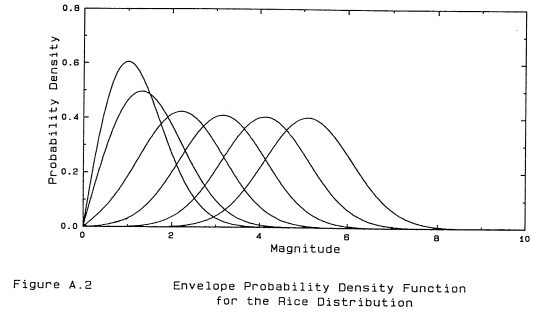
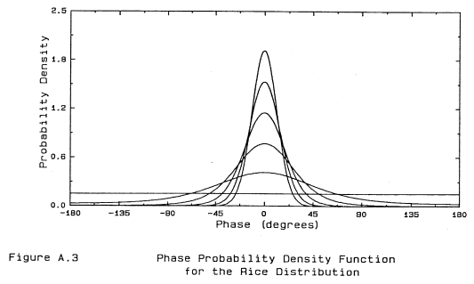
Figure A.2 and A.3 show the Rice (magnitude and phase) distributions for various values of the signal-to-noise power ratio.

• As A->0 the Rice distribution approaches the Rayleigh distribution as expected (there is no sinusoidal component.
  
• For large A the Rice distribution approaches a shifted Gaussian distribution centred at r = sigma.
  
• Again, P(r) is zero for negative r.