Case study: Visualisation Earth Mantle Core dataWritten by Paul BourkeJan 2011
The following presents some of the initial outcomes from a project to visualise Earth mantle data. The approach taken, the data sources and manipulation required will be discussed with the view to assisting others undertaking similar projects and to give an idea of the processes involved that are common across many visualisation exercises. Mantle data
The Earth Mantle data is sourced from EAPS (Earth, Atmospheric, and Planetary Sciences). The file is a plain text file with 4 columns, namely latitude, longitude, depth, and scalar value (dVp). For example the first few lines are as follows:
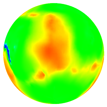
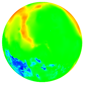
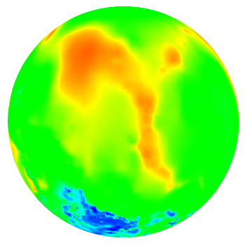
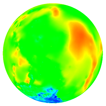
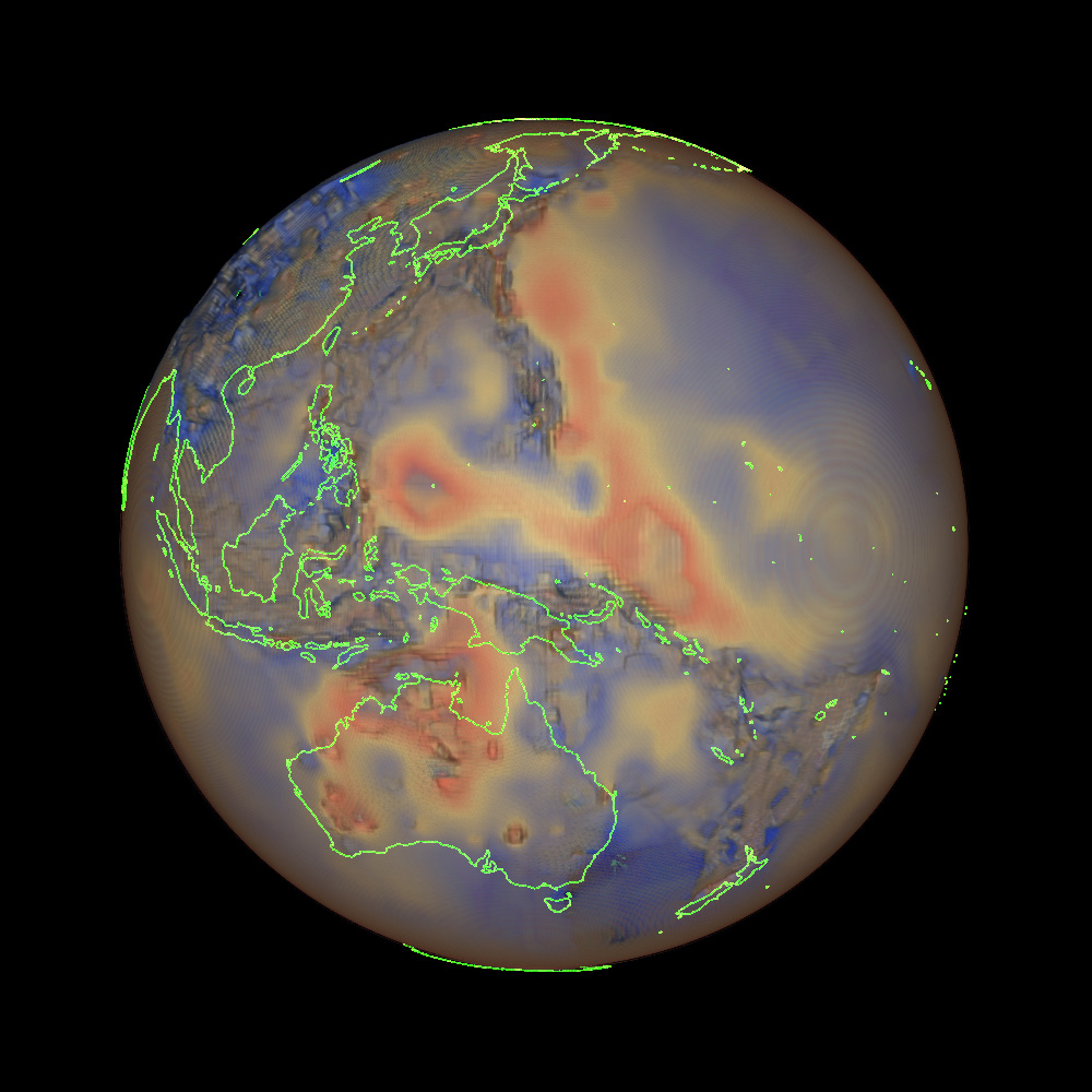
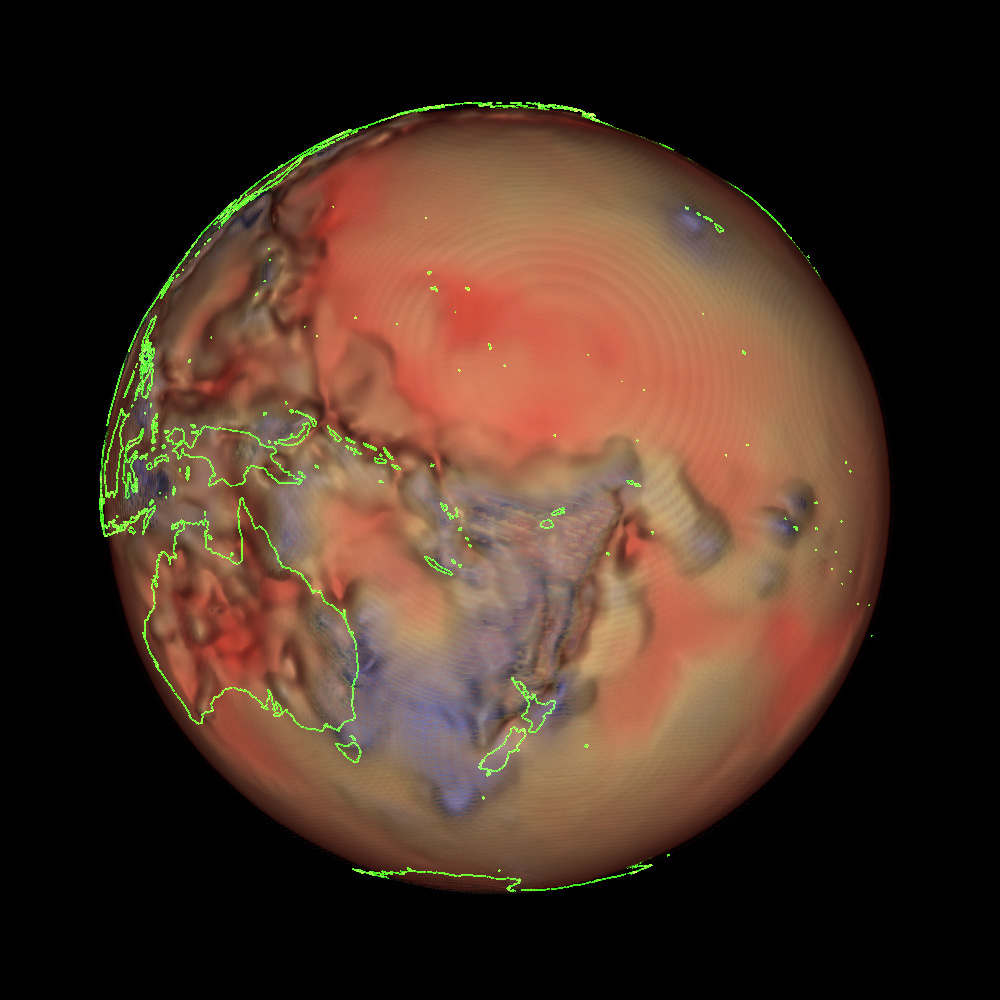
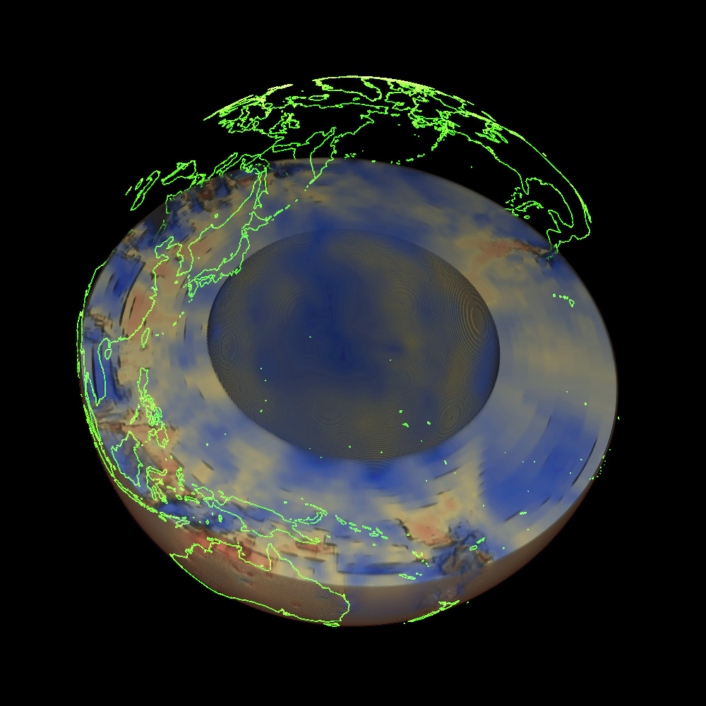
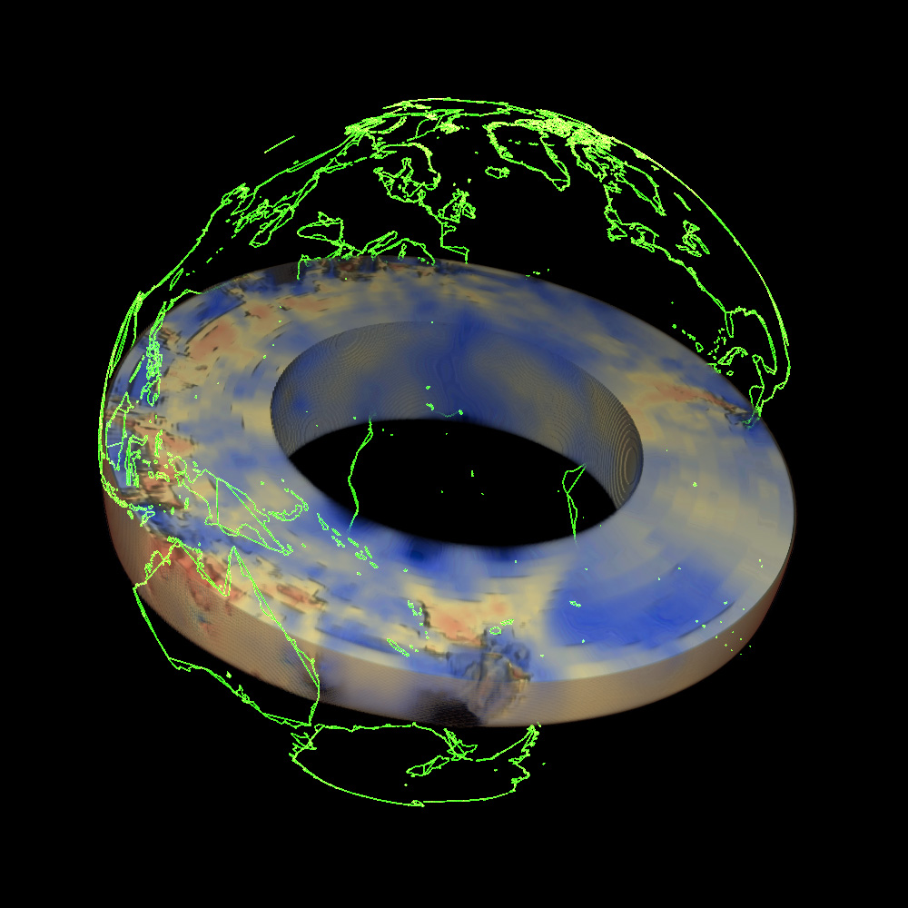
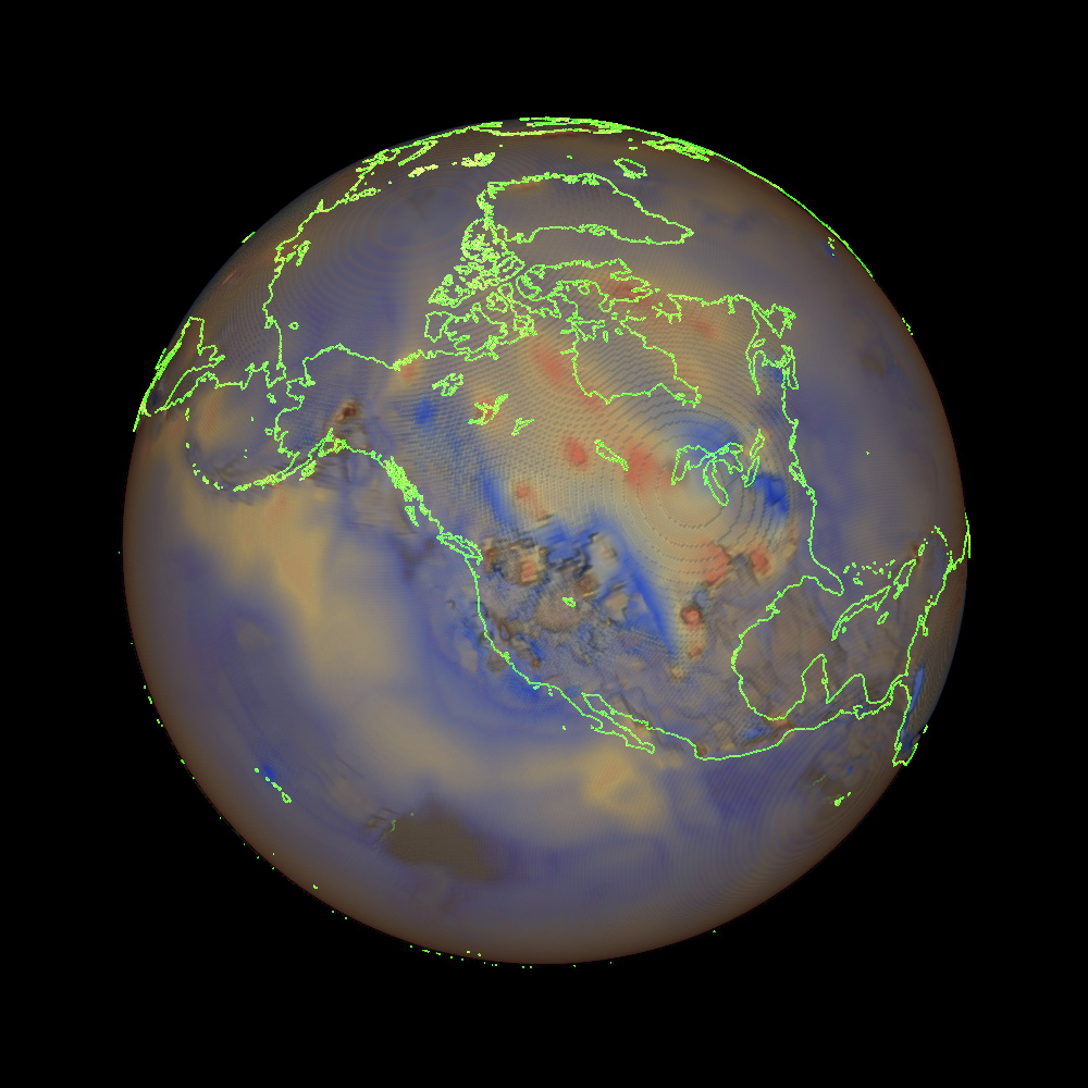
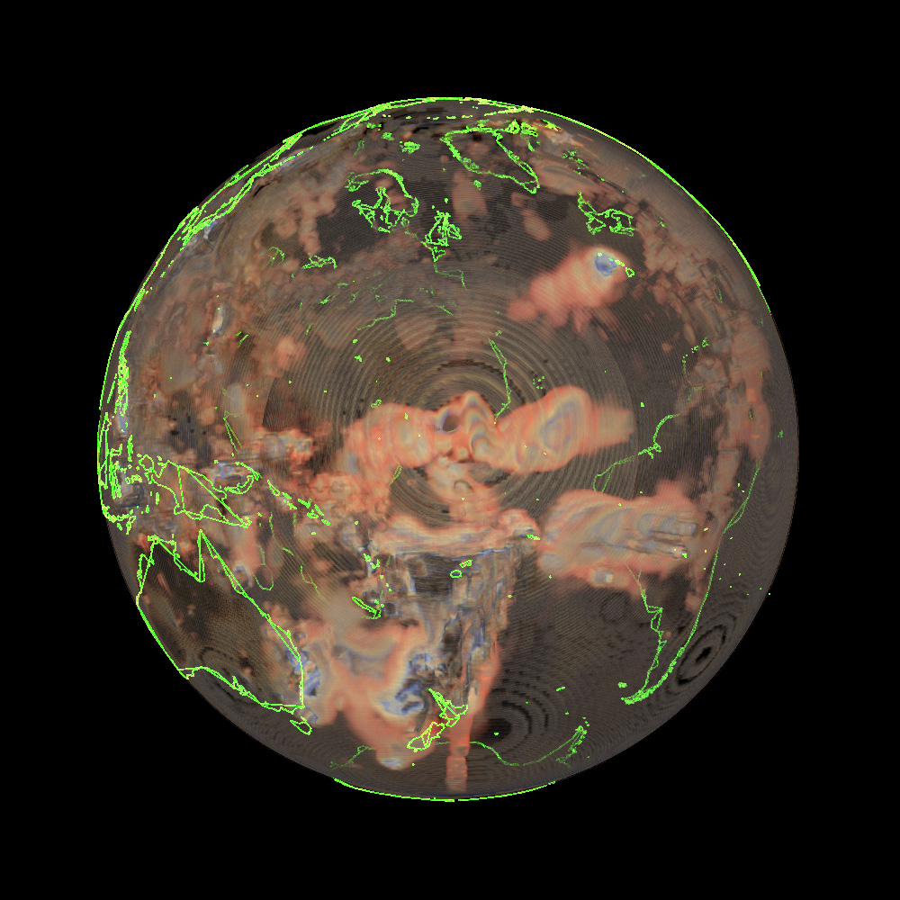
While this is essentially point data it does have a precise organisation. The data is structured in an onion peel like arrangement, data spheres of different radius. In total there are 64 different spheres ranging in depth range from 22.6km to 2868.9km (Earth radius is taken to be on average 6371km, global variation is not considered here). Each sphere is defined by 512 samples in longitude and 256 samples in latitude. Four of these spheres are shown below and the scalar value mapped to a hot-cold colour map (Note these are not all from the same view point).
Vector coastline data
In order to provide a reference to familiar structures, a coastline dataset is optionally overlaid on the volumetric data. The particular data used is from NGDC (National Geophysical Data Centre), the main reason for using this particular source was that the data is provided in an easy to parse ASCII file. The exact data is referred to as WCL (World Coast Line), the first few lines from the 1:5,000,000 dataset is as follows:
These are just polylines, the start of each is indicated by a ">" symbol, and the vertices are given in longitude and latitude. This is relatively straightforward to parse and output line segments in other formats, for example the format required by the volume visualisation software used. Note that for some reason long curve sections are often broken up into shorter pieces. The translator detects these and combines them, this assists with the subsampling in order to present a smaller more efficient series of coastal outlines to the rendering software. 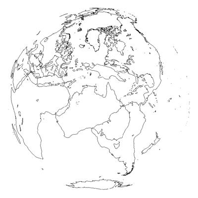
Volume rendering
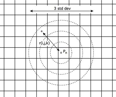
The intended means of visualising this data was though volume rendering. The software used is Drishti developed at the ANU (Australia National University). The point sample data provided for the mantle needs to be converted into a volumetric dataset. The approach taken here is to consider each voxel in the volume and determine its value as a weighted average (Gaussian weights) of the points in the neighbourhood. Stepping though each voxel and then considering each point in the mantle data (512*256*64 = 8388608 points) is clearly inefficient. Rather each point is considered in turn, its position in the volume coordinate system is determined, and then its contribution to voxels in that vicinity is calculated. Gaussian weighting is used and contributions are only made to voxels +- 3 standard deviations (user selectable parameter) away from the central voxel. The sum of the weights is also recorded and used at the end of the process to normalise the value at each voxel.
For this to be successful there is a balancing act between the resolution of the volume and the chosen standard deviation. One needs to ensure that each voxel is at least being contributed to and at the same time it is desirable if voxels are not being contributed to by too many points.
Inevitably there are aliasing and moire artefacts arising from a sphere being sampled by a square Cartesian grid. Examples of this are quite clear from the image on the last and left hand cell above. These are only reduced by increasingly higher resolution volumes.
Oceans of the EarthWritten by Paul Bourke, idea inspired by Peter Morse.February 2009
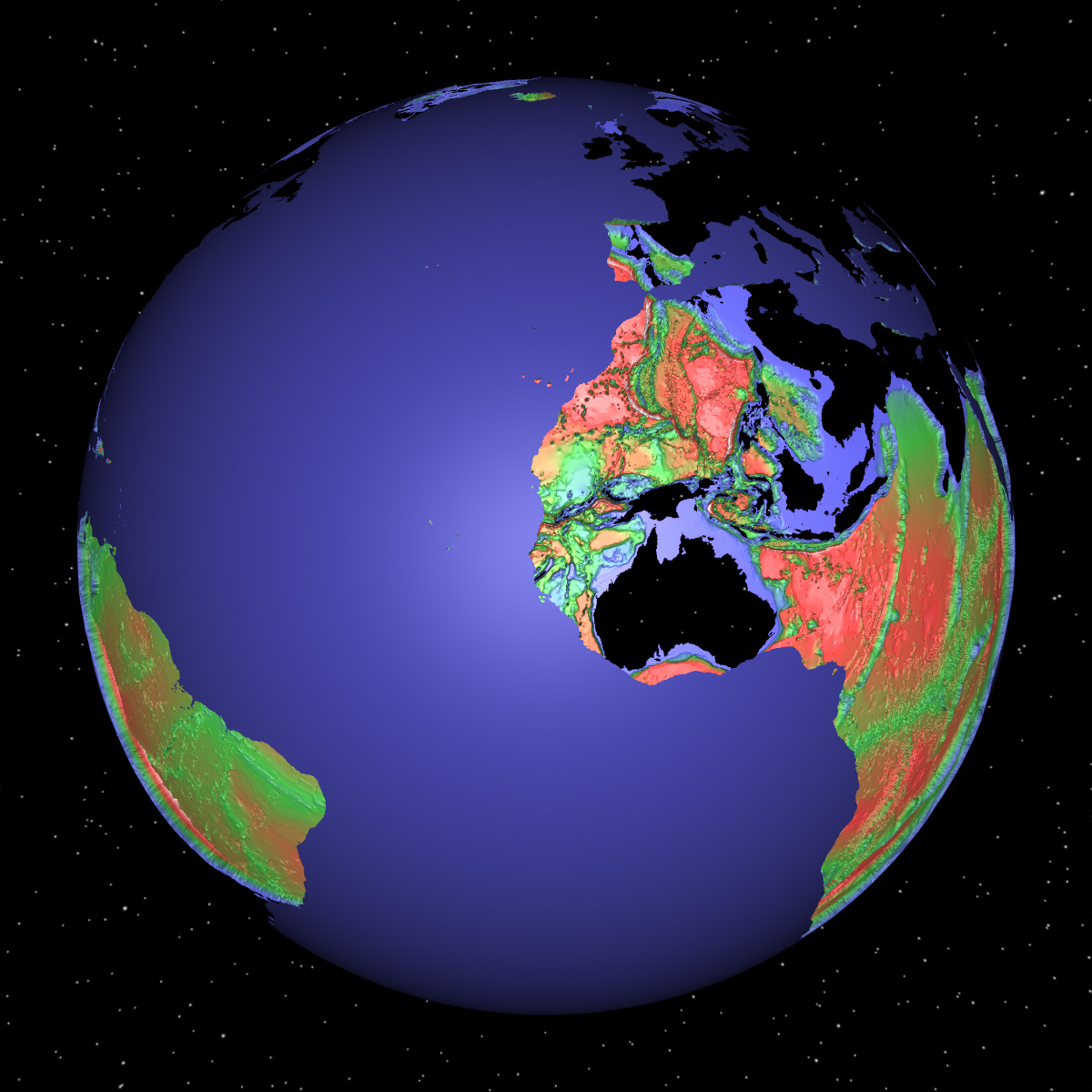
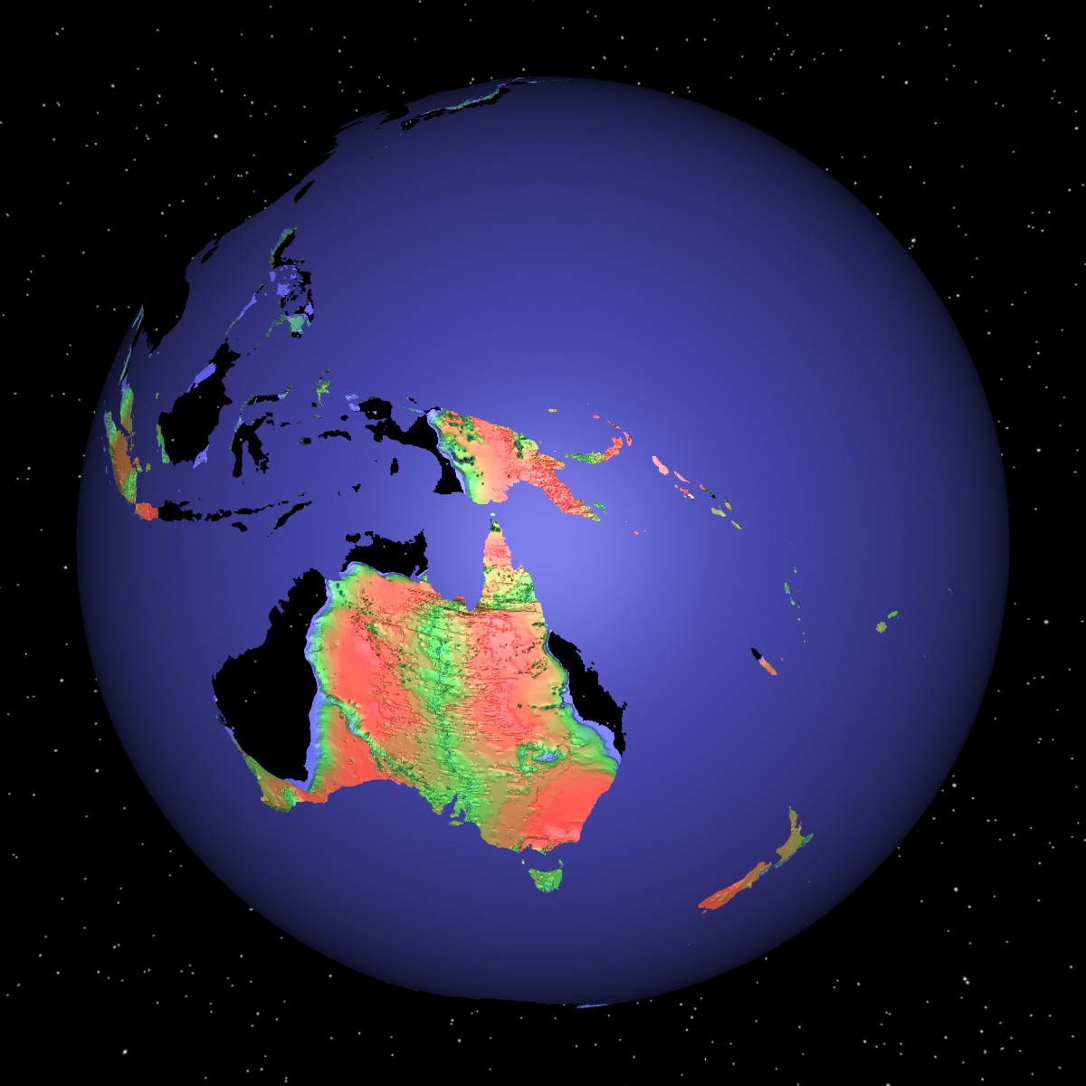
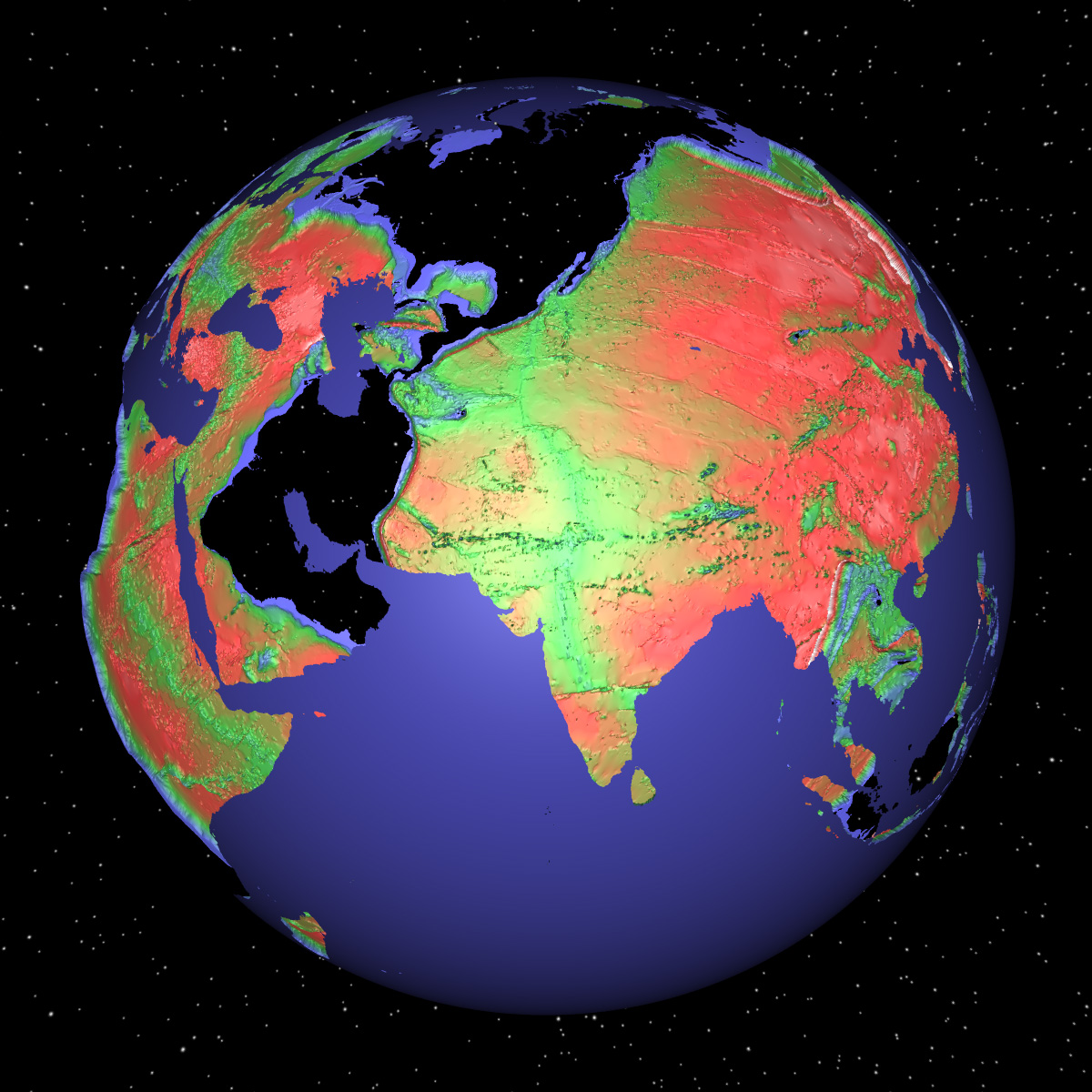
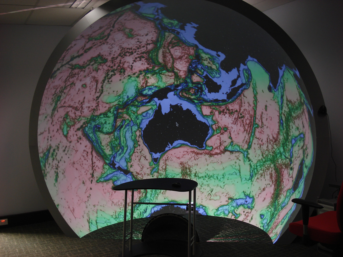
We are used to seeing the Earth from space, as maps, 3D renderings, or actual photographs. We instantly recognise the landforms, those are the areas of the Earth we occupy. But what does the Earth look like if we switch our attention to the oceans? For a being living in the oceans this is the view they would concentrate on and the land would be the unchartered and unexplored areas. In the following the land has been removed from the planet leaving just the ocean body. The data used here is derived from the GEBCO dataset, the elevation of the whole planet (including ocean bottom) at 1 minute (1/60 degree) resolution. The first image below is the Earth in the typical spherical projection, as viewed from the inside looking out. 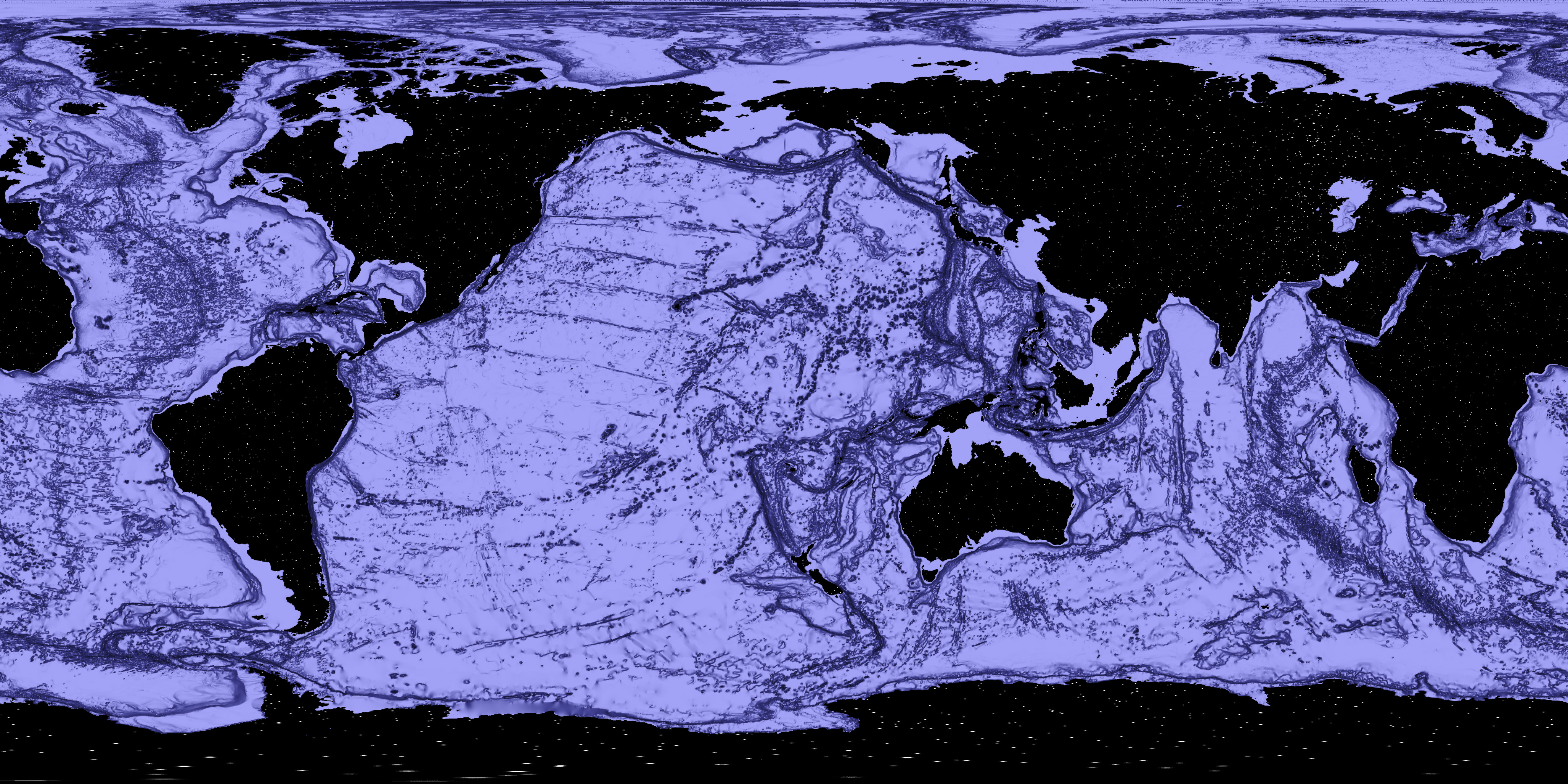 Click for 4K wide version
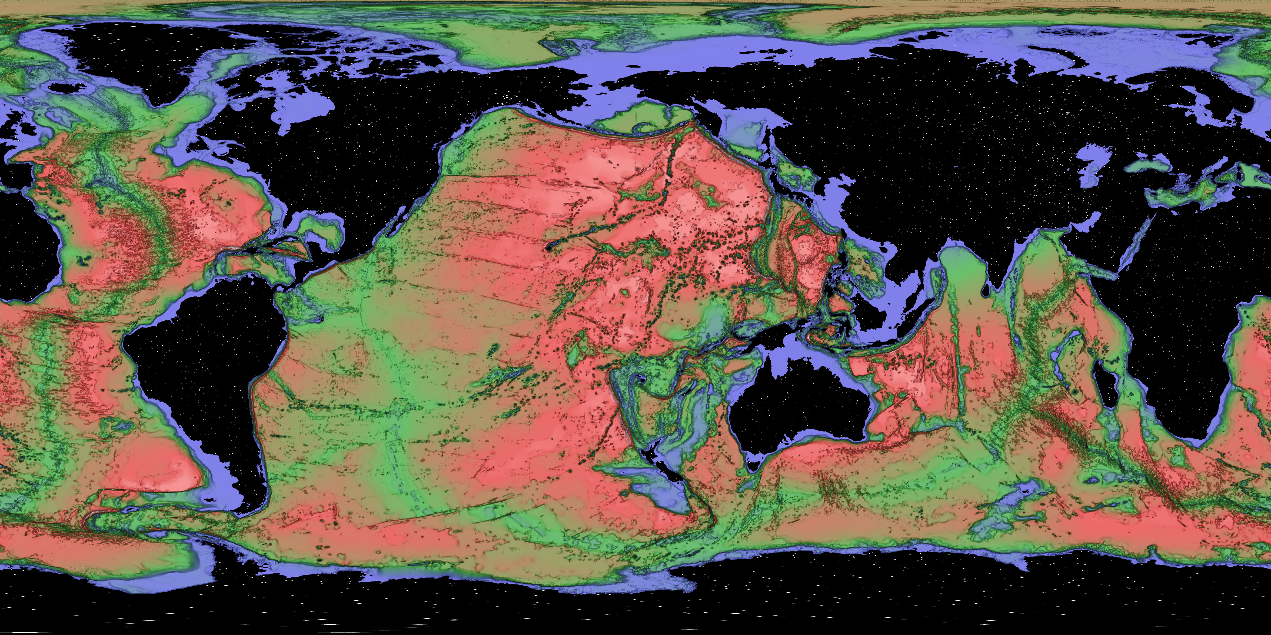
Views from space, ocean depth exaggerated by a factor of 25. Colour shading by depth, blue being shallow water and red the deepest. This QuickTime movie (ocean_spin_512.mov) is perhaps clearer than the still images.
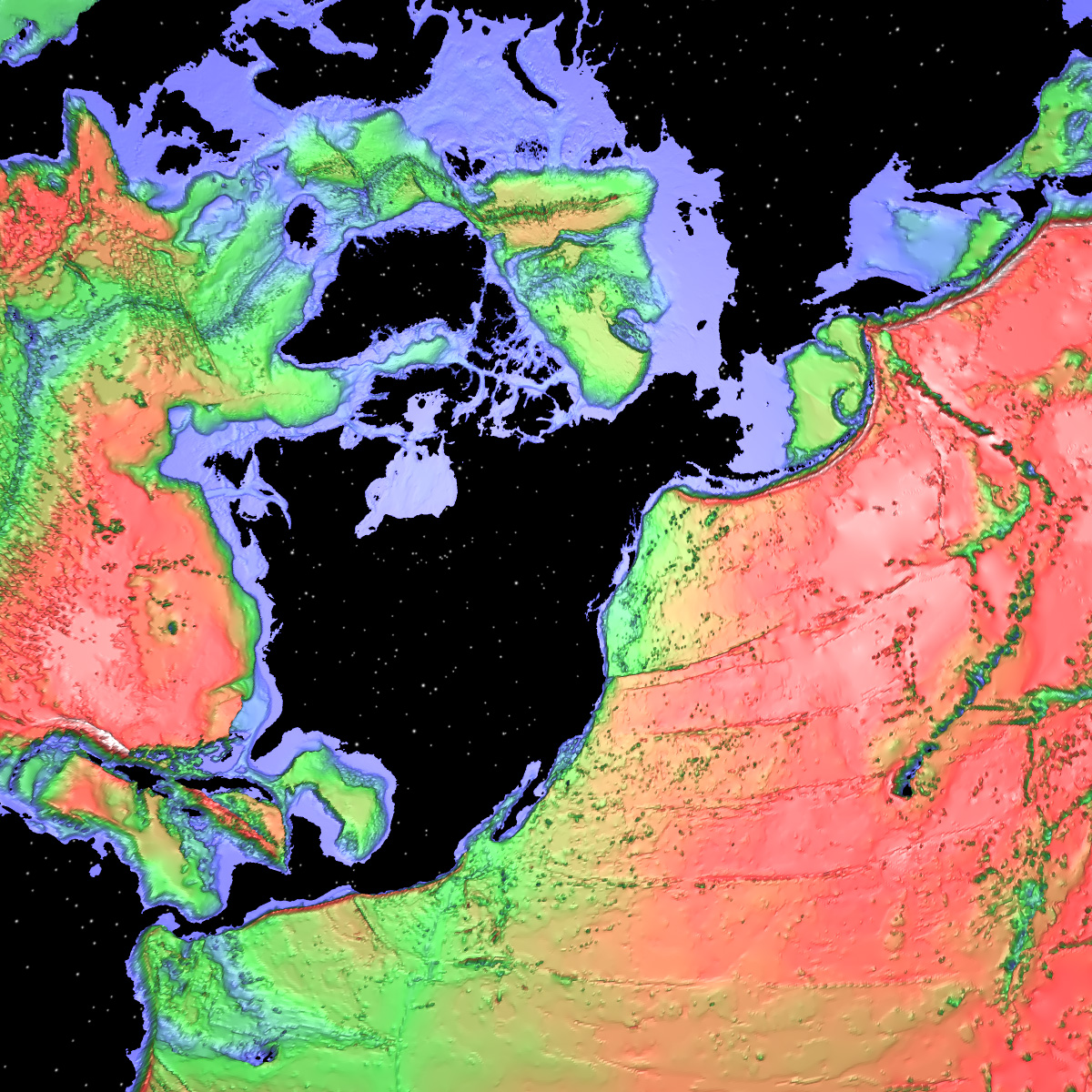
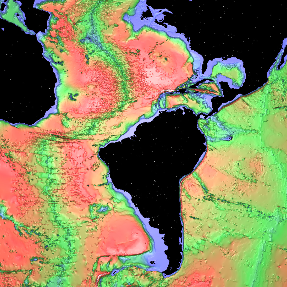
Views from within the Earths crust.
In the iDome.
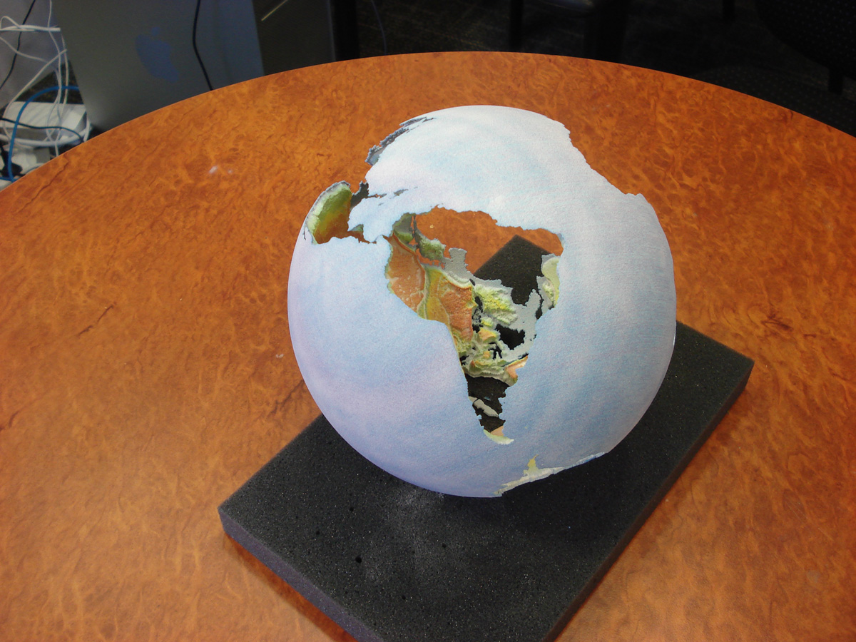
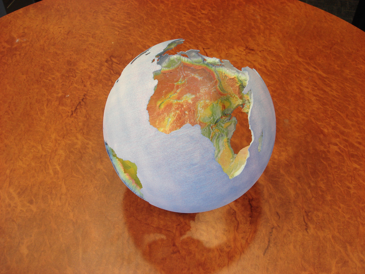
Rapid prototype using Z-Corp colour printer.
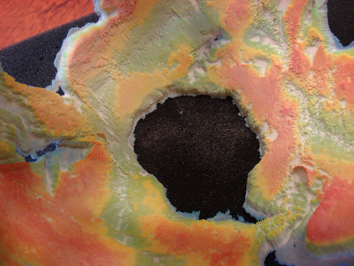
Objet 3D printer 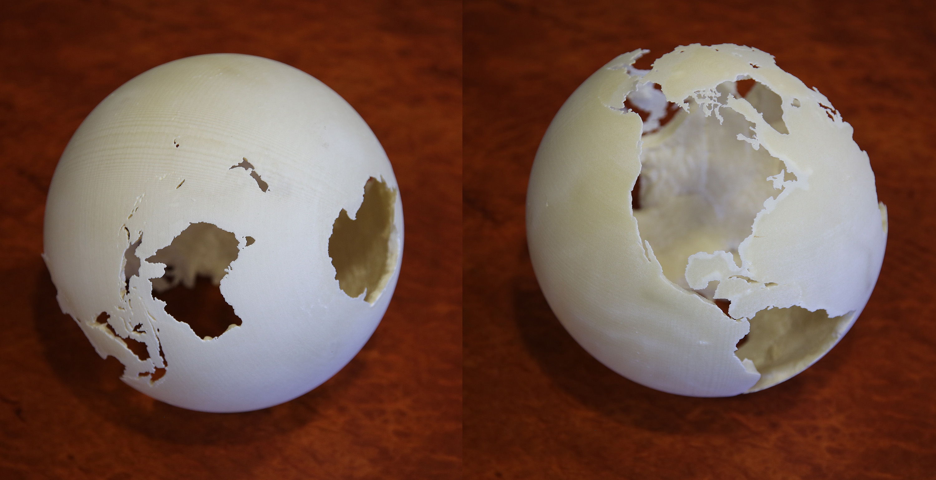
|