Approaches to Modelling the
|
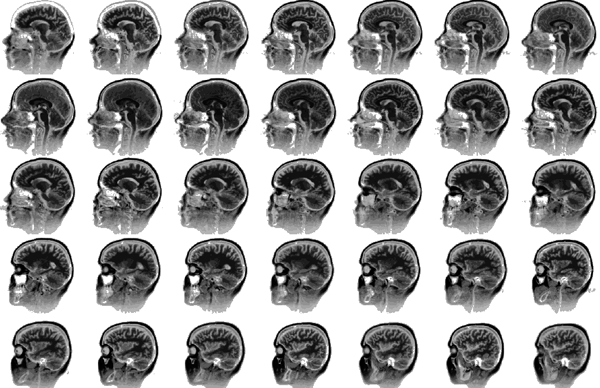
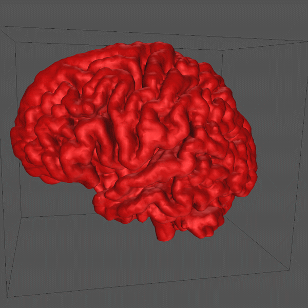
T1-weighted, GRE or MDEFT sequence, 256x256 in-plane resolution, FOV 250mm, 128 sagittal slices, 1.5mm thick, no gap. In these raw datasets we remove the outer hulls of the brain ("brain peeling"), align them with the stereotactical coordinate system and interpolate them to 1mm^3 resolution. |
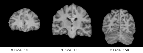


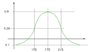
The white matter which was used to form the basis of the implicit surface controls consisted of a clear band of intensity values, from 135 -> 215.
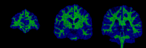
The control points are shown below in green for representative slices along each of the three orthogonal planes. Each control point is considered to be a sphere of 1mm radius so as to avoid overlapping.


Implicit surface modelling
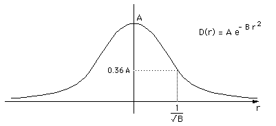
In this initial experiment the implicit surface function used is usually called blobby molecules and attributed to Jim Blinn. The field D at a distance r from a single control point is given by a Gaussian
D(r) = A e -Br2
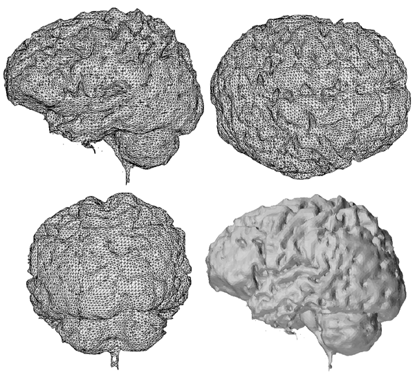
The control points were created within the white matter, an isosurface of this resulting field is an approximation to the cortex layer. In what follows the isosurface was taken to be at a level of 0.5, and A = 1.
|
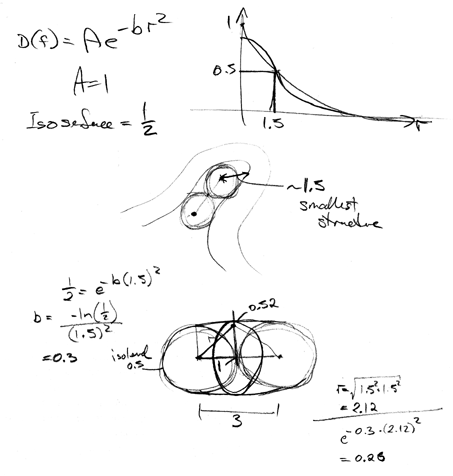
The approximate value of B can be determined by considering two
adjacent control points and the field at points between them.
B should be chosen so that the isosurface from two adjacent control
points is approximately cylindrical.
Varying B effectively creates isosurfaces at varying distance from the white matter. High B result in isosurfaces that are close to the white matter (close to the control points), low B results in more distant isosurfaces (diffuse field and smoother isosurface).... Some example for B = 0.1 to 0.25 are illustrated below.
|
|
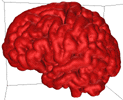 B = 0.1 |
 B = 0.15 |
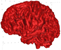 B = 0.2 |
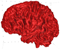 B = 0.25 |
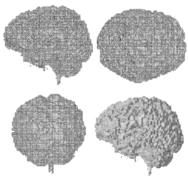
The second experiment was to consider each pixel in the MRI volume to be a control point, the intensity of the pixel being used to determine the value of A in the blobby molecule field equation. The mapping from intensity to A would be such that the white matter would result in high positive values, pixels clearly outside the cortex would result in negative values of A. It was hoped that this would help in the resolving of the sulci, preventing bridging between gyri.
|
The function used was a Gaussian with a mean of 175 and standard
deviation 40, namely
The zero crossings are approximately at intensities 114 and 235, in other words all intensities below 114 resulted in negative field contributions. |
 |
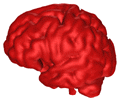 B = 0.05 |
 B = 0.10 |
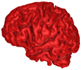 B = 0.15 |
 B = 0.25 |
Credits
The implicit surfaces were rendered by polygonising the surface using a modified marching cubes algorithm written by myself....that's another story.
The resulting polygonal surfaces were rendered using Geomview on an SGI Maximum Impact.
Movies of the MRI slices in the three planes were generated using Apple QuickTime (animation) technology.
References
James F. Blinn
A Generalization of Algebraic Surface Drawing
ACM Transactions on Graphics, July 1982
Tatsumi, H., Takaoki, E., Omura, K. and Fujito, H.
A new method for 3D reconstruction from serial sections by
computer graphics using meta-balls: reconstruction
of "Hepatoskeletal System" formed by Ito Cells in the Cod Liver
Computers and Biomedical Research, 1990
Brian Wyvill, Geoff Wyvill
Field Functions for Implicit Surfaces
Visual Computer, Issue 5 1989
F. Kruggel, G. Lohmann
Automatic Adoption of the Stereotactical Coordinate System in
MRI Datasets
Information Processing in Medical Imaging
Duncan J, Gindi G (eds.), LCNS 1230, Springer 1997.
Modelling the Surface of the Human CortexWritten by Paul BourkeFebruary 1997
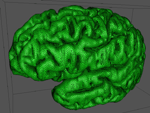
A low resolution version of this model is available in the "OFF" file format as specified by the GeomView documentation: 60000.off.gz (20000 faces) or 60000.dxf.gz Higher resolution versions are available on request.
|
|
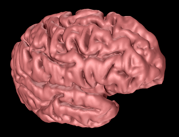
Introduction
The following informally describes a project aimed at generating a computer based surface model of a human cortex. The requirements were for a "clean" facet based model that could be used for other applications that required a surface model rather than volumetric information. In particular it was necessary to derive a model with a realistic representation of the deep sulci, a feature missing from existing surface models.
Slices
It was decided early on to use cryosection data due to its high resolution compared to MRI and other volumetric datasets available at the time.
The source for the slices used in this reconstruction is the "Human Cryotome Data" from the UCLA Laboratory of Neuro Imaging.
|
The data set contains images collected from the brain of a 76 year old normal female human cadaver. The specimen was prepared for sectioning by perfusing with 8% formalin, cryoprotecting with 10% glycerol, freezing in isopentane and dry ice and blocking in green tempera paint and 3% sucrose solution. The brain was cryosectioned at -20oC through the horizontal plane in 100um increments on a heavy duty cryomacrotome (PMV Stockholm, Sweden). The cryomacrotome was equipped with a high resolution camera for digital image capture of serial images (10242, 24-bit) collected from the cryoplaned specimen blockface at every 600um. The actual image size was measured at 18.5 cm. Data were assigned real value coordinate values in micrometers for width, height, and depth and reconstructed to a single 3D data volume. In order to place the brain into the Talairach system, different amounts of scaling were imposed on 12 rectangular regions of brain defined by vectors from the AC-PC line and the extrema. |
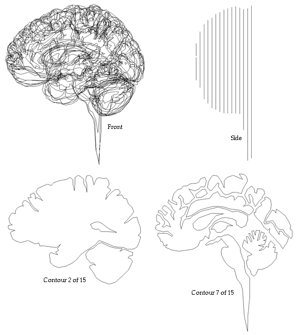
Examples of the slices

In total there were 317 slices.
Tracing
Every second section of the left hemisphere was traced with a third order B-Spline curve resulting in 168 slices. The software to perform this tracing was written in-house, it is a Macintosh program which reads a PICT file and optionally an existing spline file. The user may manipulate the spline tracing by moving, adding, or deleting control points. The spline curve is drawn interactively so the user has an immediate feedback as to the closeness of fit.
Some examples of traced sections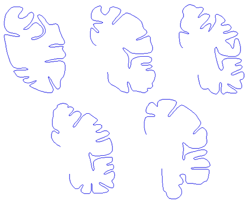
Needless to say the process of tracing each slice is tedious.
The overall dimensions for the model are
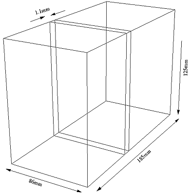
Surface Construction
The reconstruction of the cortical surface from the parallel B-Spline sections is still being considered. Linear interpolation between the spline slices was used here, it is straightforward but results in a surface with undesirable structure perpendicular to the slices. Another method evaluated involved stacking the spline sections together and spline curves are lofted perpendicular to the slice sections through the equivalent points on each section.
Improved reconstruction approaches include spline surface descriptions, implicit surfaces, and spherical harmonics.
The aim is to derive a surface description which is "well behaved" and can ideally be constructed at variable degrees of detail.
Half a dozen slices connected together are shown below.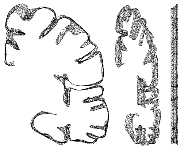
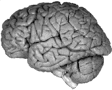
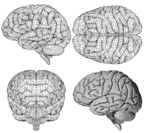
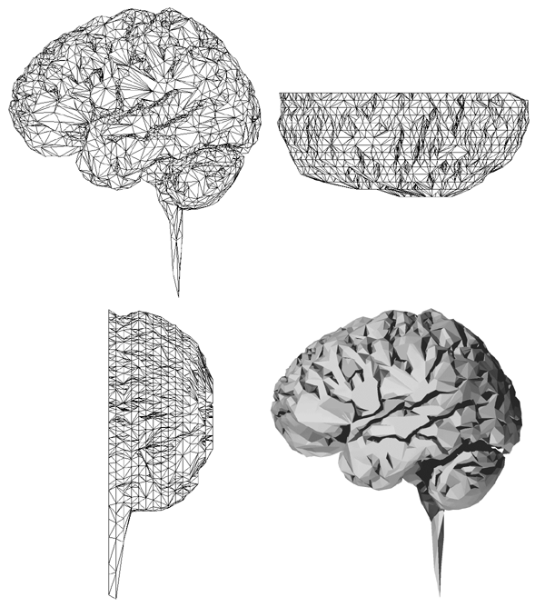
At this stage it is possible to estimate any position on the 2D spline surface and thus form triangular facet versions of the cortex surface of any desired resolution (up to some maximum as determined by the original sampling and slice thickness). The model seen at the start of this page was created by specifying a maximal edge length for the triangular facets of 1mm.
Editing/smoothing
Due to variations in the slice splines such as image registrations errors, the final reconstructed surface has undesirable vertical features (see left image below). A standard relaxation filter was passed over the surface to smooth it out, the effect is shown below.
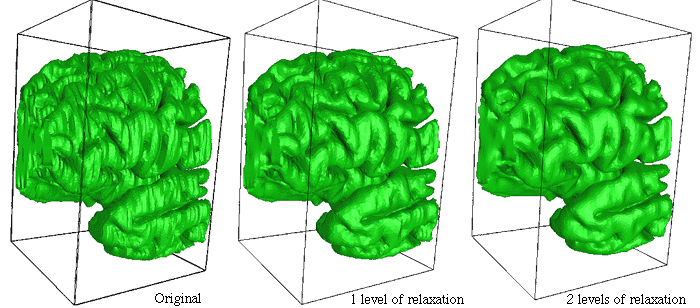
The algorithm used is applied repeatedly depending on the degree of smoothing required, two iterations were used to create the final cortical model seen at the top of this page.
|
All the software required for the above was written by myself, The rendering was performed using Geomview on an SGI Max Impact. |
Images of fibres in a model of the cortexWritten and created by Paul BourkeMay 1997 |

|
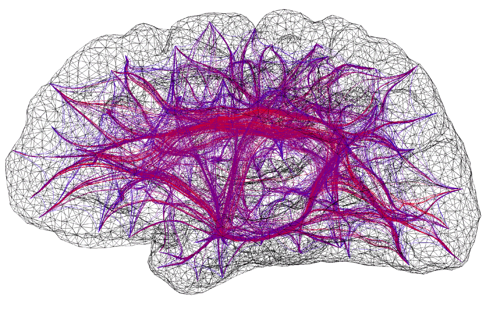
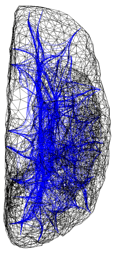
Illustration of a computer generated connectivity between discrete areas on a human cortex. Two modelling exercises have been combined in this illustration; the formation of a realistic surface representation of the human cortex and the result of a simulation to derive pathways by which fibre bundles connect surface patches.
|
Generating a realistic surface representation of the human cortex
involves a reconstruction from geometric data acquired from a real
cortex. A common approach is to use MRI scans which come in the
form of a number of 2 dimensional slices (images) through the 3
dimensional volume. While there may be sufficient resolution within
a slice, the resolution perpendicular to the slices is much poorer
resulting in inadequate spatial sampling in that dimension. It is
thus not possible, or at least very difficult, to get a realistic
reconstruction of deep sulci using MRI data. The approach taken
here was to reconstruct the surface geometry from cryosection
slices for which there is significantly better resolution both
within a slice and between slices. The cryosection data was
sourced from the UCLA Laboratory of Neuro Imaging, each slice
is separated by 0.6mm and was digitally photographed at 1000x1000
pixel resolution. The upper cortical surface was traced using a
mixture of automatic and manual procedures to form ribs over
which 2 dimensional splines were lofted. This parametric form
of the cortical surface can be sampled at any user selected
resolution to give simpler surface representations approximated
by triangular facets.
The cortical simulation software being developed within the Brain Dynamics Laboratory requires information on how small areas (patches) on the cortex are coupled together, that is, the strength of coupling and delay between any two patches. Both of these parameters are functions of the distance of the pathway taken by the fibre bundle. The pathways were derived by modelling the cortex as a positively charged surface and a fibre as a collection of positively charged springs connected end-to-end along the pathway. The fibre path is found by iteratively relaxing the spring model to find the route of minimum potential energy. This model gives the desired properties we chose for the fibre pathways, the fibres are roughly perpendicular to the surface of the cortex, they attempt to find the shortest route between patches, and they don't intersect the surface or each other. For this type of whole brain macroscopic simulation the surface of the cortex was split into about 600 patches. Fibres from any one patch can potentially connect to any other patch resulting in a huge number of fibres. In practice however, the very long or convoluted pathways have a very small coupling value and can be safely pruned. Additional long range fibres representing the superior longitudinal fasciculus, inferior longitudinal fasciculus, and unicinate fasciculus were also added to the model. These additional longer range fibres have their pathways determined by similar techniques but their coupling strength is based upon a different function of distance.
|
|
