Cross CorrelationAutoCorrelation -- 2D Pattern Identification
Written by Paul Bourke
Cross correlation is a standard method of estimating the degree to which two series are correlated. Consider two series x(i) and y(i) where i=0,1,2...N-1. The cross correlation r at delay d is defined as 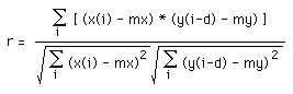 Where mx and my are the means of the corresponding series. If the above is computed for all delays d=0,1,2,...N-1 then it results in a cross correlation series of twice the length as the original series. 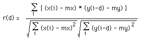 There is the issue of what to do when the index into the series is less than 0 or greater than or equal to the number of points. (i-d < 0 or i-d >= N) The most common approaches are to either ignore these points or assuming the series x and y are zero for i < 0 and i >= N. In many signal processing applications the series is assumed to be circular in which case the out of range indexes are "wrapped" back within range, ie: x(-1) = x(N-1), x(N+5) = x(5) etc The range of delays d and thus the length of the cross correlation series can be less than N, for example the aim may be to test correlation at short delays only. The denominator in the expression above serves to normalise the correlation coefficients such that -1 <= r(d) <= 1, the bounds indicating maximum correlation and 0 indicating no correlation. A high negative correlation indicates a high correlation but of the inverse of one of the series.
Source code Sample C source to calculate the correlation series with no data wrapping. The two series are x[], and y[] of "n" points. The correlation series is calculated for a maximum delay of "maxdelay".
   int i,j
   double mx,my,sx,sy,sxy,denom,r;

   /* Calculate the mean of the two series x[], y[] */
   mx = 0;
   my = 0;
   for (i=0;i<n;i++) {
      mx += x[i];
      my += y[i];
   }
   mx /= n;
   my /= n;

   /* Calculate the denominator */
   sx = 0;
   sy = 0;
   for (i=0;i<n;i++) {
      sx += (x[i] - mx) * (x[i] - mx);
      sy += (y[i] - my) * (y[i] - my);
   }
   denom = sqrt(sx*sy);

   /* Calculate the correlation series */
   for (delay=-maxdelay;delay<maxdelay;delay++) {
      sxy = 0;
      for (i=0;i<n;i++) {
         j = i + delay;
         if (j < 0 || j >= n)
            continue;
         else
            sxy += (x[i] - mx) * (y[j] - my);
         /* Or should it be (?)
         if (j < 0 || j >= n)
            sxy += (x[i] - mx) * (-my);
         else
            sxy += (x[i] - mx) * (y[j] - my);
         */
      }
      r = sxy / denom;

      /* r is the correlation coefficient at "delay" */

   }
If the series are considered circular then the source with the same declarations as above might be
   /* Calculate the mean of the two series x[], y[] */
   mx = 0;
   my = 0;
   for (i=0;i<n;i++) {
      mx += x[i];
      my += y[i];
   }
   mx /= n;
   my /= n;

   /* Calculate the denominator */
   sx = 0;
   sy = 0;
   for (i=0;i<n;i++) {
      sx += (x[i] - mx) * (x[i] - mx);
      sy += (y[i] - my) * (y[i] - my);
   }
   denom = sqrt(sx*sy);

   /* Calculate the correlation series */
   for (delay=-maxdelay;delay<maxdelay;delay++) {
      sxy = 0;
      for (i=0;i<n;i++) {
         j = i + delay;
         while (j < 0)
            j += n;
         j %= n;
         sxy += (x[i] - mx) * (y[j] - my);
      }
      r = sxy / denom;

      /* r is the correlation coefficient at "delay" */

   }
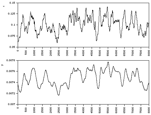
ExampleThe following shows two time series x,y.
The cross correlation series with a maximum delay of 4000 is shown below. There is a strong correlation at a delay of about 40. 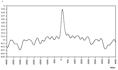
When the correlation is calculated between a series and a lagged version
of itself it is called autocorrelation. A high correlation is likely to
indicate a periodicity in the signal of the corresponding time duration.
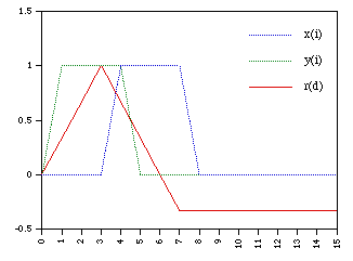
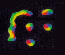
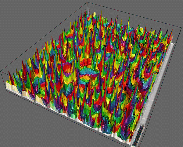
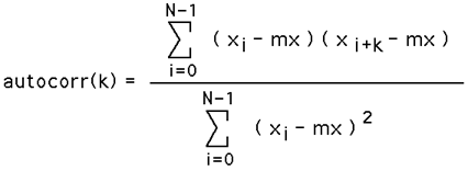 Where mx is the mean of the series. When the term i+k extends past the length of the series N two options are available. The series can either be considered to be 0 or in the usual Fourier approach the series is assumed to wrap, in this case the index into the series is (i+k) mod N. If the correlation coefficient is calculated for all lags k=0,1,2...N-1 the resulting series is called the autocorrelation series or the correlogram. The autocorrelation series can be computed directly as above or from the Fourier transform as That is, one can compute the autocorrelation series by transforming the series into the frequency domain, taking the modulus of each spectral coefficient, and then performing the inverse transform. Note that depending on the normalisation used with the particular FFT algorithm there may need to be a scaling by N. This method for computing the auto correlation series is particularly useful for long series where the efficiency of the Fast Fourier Transform can significantly reduce the time required to compute the autocorrelation series. Note that this is a special case of the expression for calculating the cross correlation using Fourier transforms. The Fourier transform of the cross correlation function is the product of the Fourier transform of the first series and the complex conjugate of the Fourier transform of the second series. 2D Pattern Identification using Cross CorrelationOne approach to identifying a pattern within an image uses cross correlation of the image with a suitable mask. Where the mask and the pattern being sought are similar the cross correlation will be high. The mask is itself an image which needs to have the same functional appearance as the pattern to be found. Consider the image below in black and the mask shown in red. The mask is centered at every pixel in the image and the cross correlation calculated, this forms a 2D array of correlation coefficients. 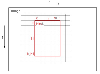 The form of the un-normalised correlation coefficient at position (i,j) on the image is given by  The peaks in this cross correlation "surface" are the positions of the best matches in the image of the mask. Issues
The maximum cross correlation for all angles and for each of the two masks is retained for each position. This maximum cross correlation surface with the image mapped onto it is 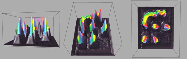
The resulting surface where the height is proportional to the maximum correlation coefficient across all angles and for the mirror of the masks is 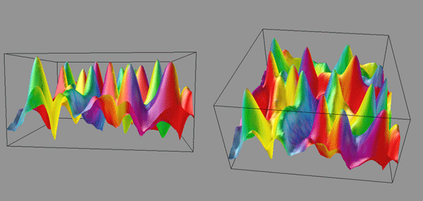
The width and relative height of the correlation peaks can be improved by matching the dimensions of the mask with those of the features being sought in the image. For example, if the size of the mask is smaller and radial as below
then the peaks are significantly narrower. 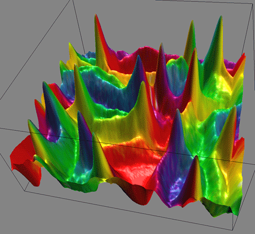
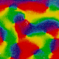
The above is an example over a relatively small portion of the whole image. The entire surface is 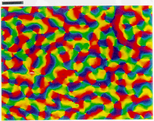
The maximum cross correlation image (white = high correlation, black = low correlation) 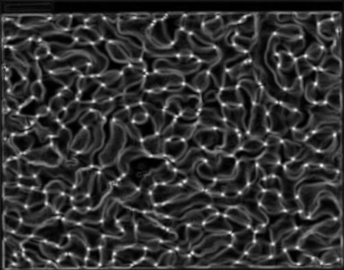
And finally the surface shown in 3D with the original image mapped onto it 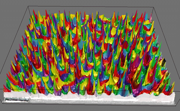
|