Auto-regression Analysis (AR)Written by Paul BourkeCredits for source code: Alex Sergejew, Nick Hawthorn, Rainer Hegger. November 1998
IntroductionAn autoregressive model (AR) is also known in the filter design industry as an infinite impulse response filter (IIR) or an all pole filter, and is sometimes known as a maximum entropy model in physics applications. There is "memory" or feedback and therefore the system can generate internal dynamics. The definition that will be used here is as follows
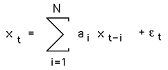 where ai are the auto-regression coefficients, xt is the series under investigation, and N is the order (length) of the filter which is generally very much less than the length of the series. The noise term or residue, epsilon in the above, is almost always assumed to be Gaussian white noise. Verbally, the current term of the series can be estimated by a linear weighted sum of previous terms in the series. The weights are the auto-regression coefficients. The problem in AR analysis is to derive the "best" values for ai given a series xt. The majority of methods assume the series xt is linear and stationary. By convention the the series xt is assumed to be zero mean, if not this is simply another term a0 in front of the summation in the equation above. SolutionsA number of techniques exist for computing AR coefficients. The main two categories are least squares and Burg method. Within each of these there are a few variants, the most common least squares method is based upon the Yule-Walker equations. MatLab has a wide range of supported techniques, note that when comparing algorithms from different sources there are two common variations, first is whether or not the mean is removed from the series, the second is the sign of the coefficients returned (this depends on the definition and is fixed by simply inverting the sign of all the coefficients). The most common method for deriving the coefficients involves multiplying the definition above by xt-d, taking the expectation values and normalising (see Box and Jenkins, 1976) gives a set of linear equations called the Yule-Walker equations that can be written in matrix form as 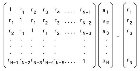 where rd is the autocorrelation coefficient at delay d. Note: the diagonal is r0 = 1. ExampleThe following example is presented with some degree of detail in order to allow replication and comparison of the results with other packages. The data is 1000 samples from a sum of 4 sinusoids and is provided here. The data looks like this 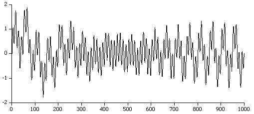 While not particularly useful, an order 1 AR analysis gives a coefficient of 0.941872, this is not totally surprising as it is saying that by only looking at one term in the series the next term in the series is probably almost the same, ie: xt+1 = 0.941872 * xt The following table gives the coefficients for a number of model orders for the example above.
      | Coefficients
Order |     1         2        3         4         5        6        7        8
----- | -------- --------- -------- --------- --------- --------- -------- ---------
1     | 0.941872
2     | 1.826156 -0.938849
3     | 2.753231 -2.740306 0.985501
4     | 3.736794 -5.474295 3.731127 -0.996783
8     | 4.259079 -6.232740 2.107323  2.969714 -1.421269 -2.591832 2.614633 -0.704923
As the order increases the estimates generally improve (this may not necessarily be so for noisy data when employing large AR orders!). It is often useful to plot the RMS error between the series estimated by the AR coefficients and the actual series. An example for the above case is shown below 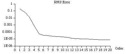
As is typical in AR analysis, the RMS error drops away very fast and then evens out. Special casesWhite noiseThe RMS error stays constant as the AR order is increased.
Constant Most AR routines fail in this case even though the solution is straightforward (a1 = 1, else ai = 0). A singular matrix results for the least squares formulation. Test 1Perhaps the best way to test code for computing AR coefficients is to generate artificial series with known coefficients and then check that the AR calculation gives the same results. For example one can generate the series where a1 = 1.4, a2 = -0.7, a3 = 0.04, a4 = 0.7, a5 = -0.5. AR analysis using a degree of 5 should yield the same coefficients as those used to generate the series. The data for this series is available here and is illustrated below: 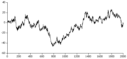 Test 2 This test case is of order 7, the coefficients are: The raw series can be found here and the data is plotted below. 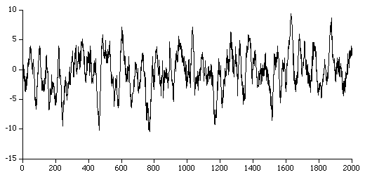 Test 3 This test case is of order 2, the coefficients are: a1 = 1.02, a2 = -0.53, The raw series can be found here and the data is plotted below. 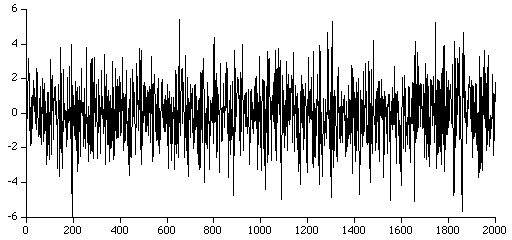
Selecting the order of the modelThere is no straightforward way to determine the correct model order. As one increases the order of the model the root mean square RMS error generally decreases quickly up to some order and then more slowly. An order just after the point at which the RMS error flattens out is usually an appropriate order. There are more formal techniques for choosing the model order, the most common of which is the Akaike Information Criterion. Source codeSource code for computing AR coefficients is available here. Two algorithms are available, the least squares method and the Burg Maximum Entropy method. A modified version (burg.c) of the Burg method (C style zero index arrays) contributed by Paul Sanders. |