Saving images from OpenGL applicationsWritten by Paul Bourke
It is not uncommon that one wants to be able to create and save images from an OpenGL application. This might be for promotional purposes, a WWW page, documentation, creating frames for an animation etc. This short note gives a simple example on how this can be done, making it elegant and suited to your own needs is left as an exercise. Window DumpThe first example creates a raw image file but of course it can be modified to write any image format. The source code is given here: WindowDump(). The key parts are setting the read buffer correctly, glReadBuffer(GL_BACK_LEFT); and reading the buffer image glReadPixels(0,0,width,height,GL_RGB,GL_UNSIGNED_BYTE,image); Note
One restriction of the above method is that one is limited to screen resolution, how does one create a higher resolution image? One way to handle this is to render the scene N times (N = 4 in the following example), each time the viewport is set so as to capture the appropriate subimage.
   if (dobigdump) {
      glMatrixMode(GL_PROJECTION);
      glLoadIdentity();
      CreateTheProjection();                /* - Application Specific - */
      for (i=0;i<4;i++) {
         for (j=0;j<4;j++) {
            fprintf(stderr,"Frame (%d,%d)\n",i,j);
            ClearTheBuffers();              /* - Application Specific - */
            glViewport(-i*width,-j*height,4*width,4*height);
            glMatrixMode(GL_MODELVIEW);
            glDrawBuffer(GL_BACK);
            glLoadIdentity();
            gluLookAt(vp.x,vp.y,vp.z,focus.x,focus.y,focus.z,up.x,up.y,up.z);
            MakeLighting();
            MakeMaterial();
            DrawTheModel();                 /* - Application Specific - */
            WindowDump();
            glutSwapBuffers();
         }
      }
      dobigdump = FALSE;
   }
Note
Distributed OpenGL RenderingWritten by Paul BourkeJuly 1996 Introduction The following outlines a method of distributing an OpenGL model across a number of computers each with their own OpenGL rendering card. The OpenGL model might be distributed using MPI from a controlling machine (that need not have OpenGL capabilities). Each of the slaves render a subset of the geometry and send their draw buffers and depth buffers back to the controlling machine. These images are combined according to the values in their depth buffers. The problemWhile tremendous performance improvements (especially price performance) are being made in OpenGL cards, there will always be geometric models that bring the best card to it's knees. For example, a high performance card might be able to render 15 million triangular facets per second. For interactive rates of 20 frames per second this means that one can display geometry with 750,000 polygons, if one wishes to render in stereo that drops to models with 375,000 triangular polygons. While this might seem a large number of polygons for those in the virtual reality or games market, it is a relatively low polygon count for many scientific visualisation applications. As an example, the terrain model shown below of Mars contains over 11 million triangular polygons.  Possible Solution A solution that follows the trends in cluster computing is to distribute the OpenGL rendering load among a number of machines. Fortunately, OpenGL maintains a depth buffer and this buffer is accessible to the programmer using glReadPixels(). The idea then is to split up the geometry making up the scene and distribute each piece to one OpenGL card, generally each card will be in a separate computer. Each card will then only need to render a subset of the geometry. For example, for a terrain model it is quite easy to split the polygons up evenly (the splitting of the geometry so that each OpenGL card is evenly loaded is not always trivial) so if there are N machines, each one only handles 1/N of the total number of polygons. Each OpenGL card then renders it's portion of the geometry and sends the image and depth buffer to be merged into the final image. The logic for this is straightforward, set a pixel in the final image to the pixel in the subimage which has the smallest depth value, ie: is closest to the camera. Example
Limitation The fundamental problem with this technique is bandwidth. Consider rendering a 800 x 600 RGB model at 20 frames per second. There are 3 bytes for each image pixel and 4 bytes for each depth buffer pixel. So to transmit an image/depthbuffer pair from one machine to another requires (3 + 4) * 800 * 600 bytes or just over 3MB. For interactive performance at 20 frames per second this requires a bandwidth of 60MB per second which is clearly more than the capabilities of all but the very highest performance networks. To make matters worse even higher bandwidth is required the more OpenGL cards participate in the rendering although bandwidth bottlenecks can be reduced by arranging the OpenGL cards/machines in a tree structure and combining the image/depthbuffer pairs as the image pieces move up the tree.  References Sepia: Scalable 3D compositing using PCI Pamette. Laurent Moll, Alan Heinrich, Mark Shand. Compaq Computer Corporation, Systems Research Center, Palo Alto, California, USA.
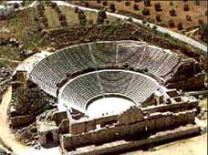
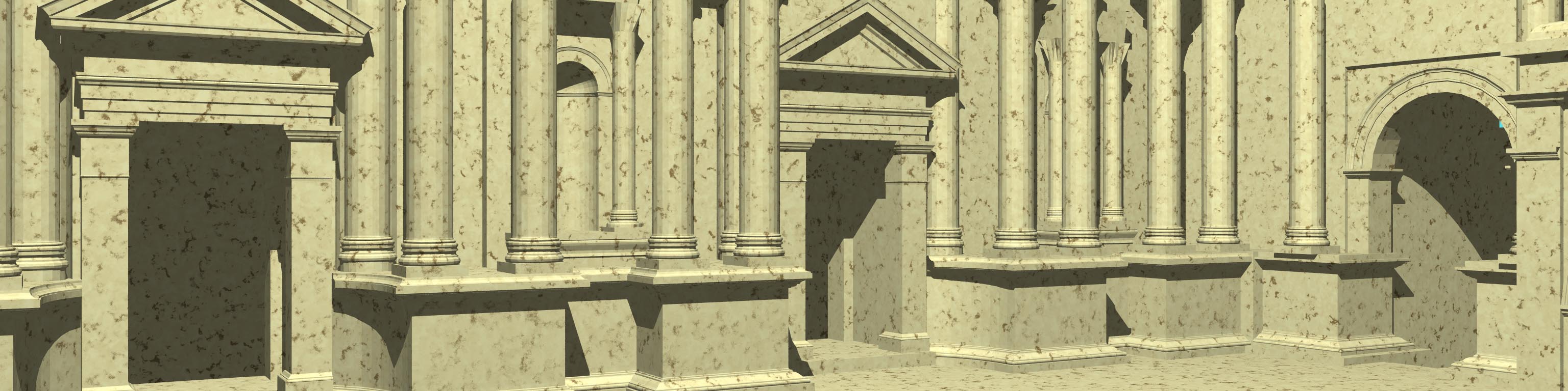
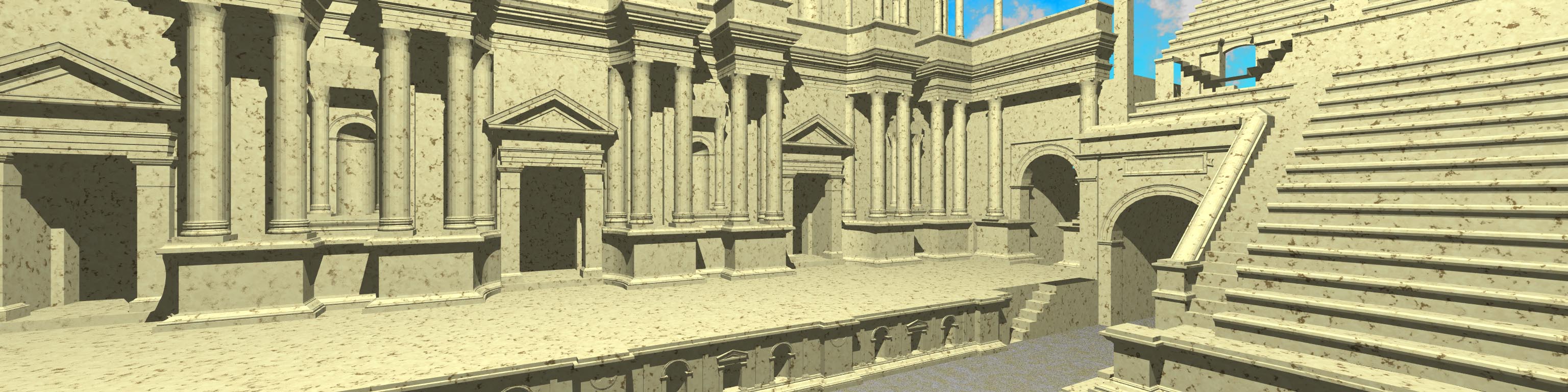
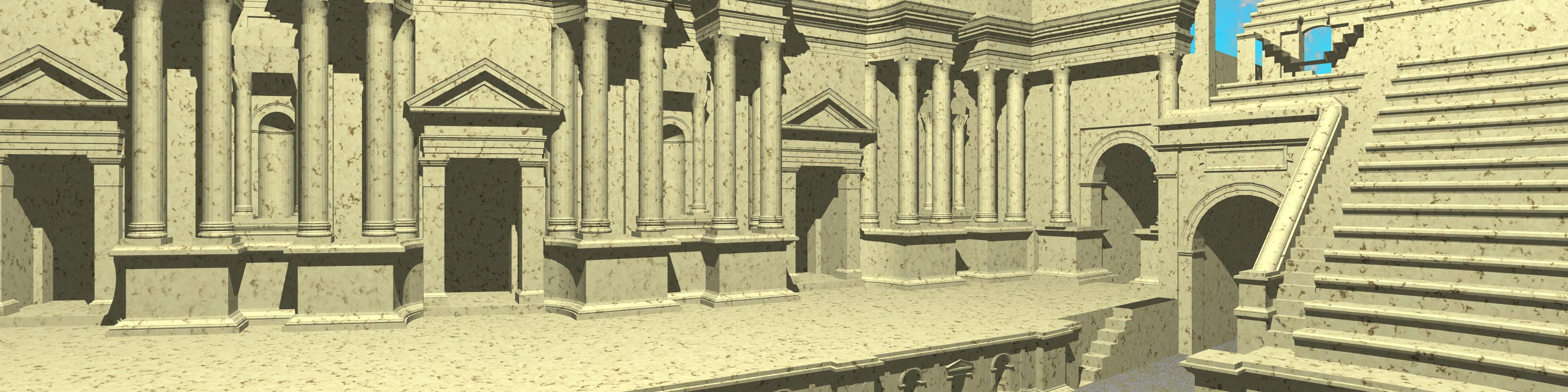
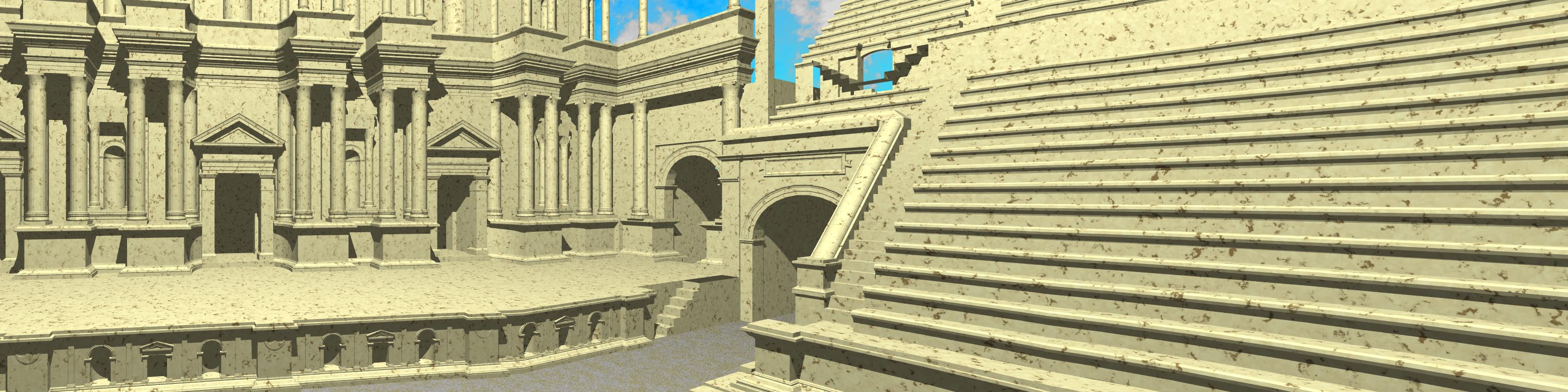
The following discusses an attempt to translate an Architectural model from AutoCAD so that it can be explored interactively in OpenGL. The AutoCAD model was supplied courtesy of the Melbourne University School of Architecture and like many models of this kind it was designed solely for AutoCAD and not for interactive rendering. The geometry was exported "as is", the aim was to explore how far one could go with automatic measures. Two wire frame shots of the model are shown below. 
Note that there are a large number of facets, about 250,000. The vast majority were 3 vertex polygons, this is mostly due to the exporter for WRL files which was used to extract the geometry. 
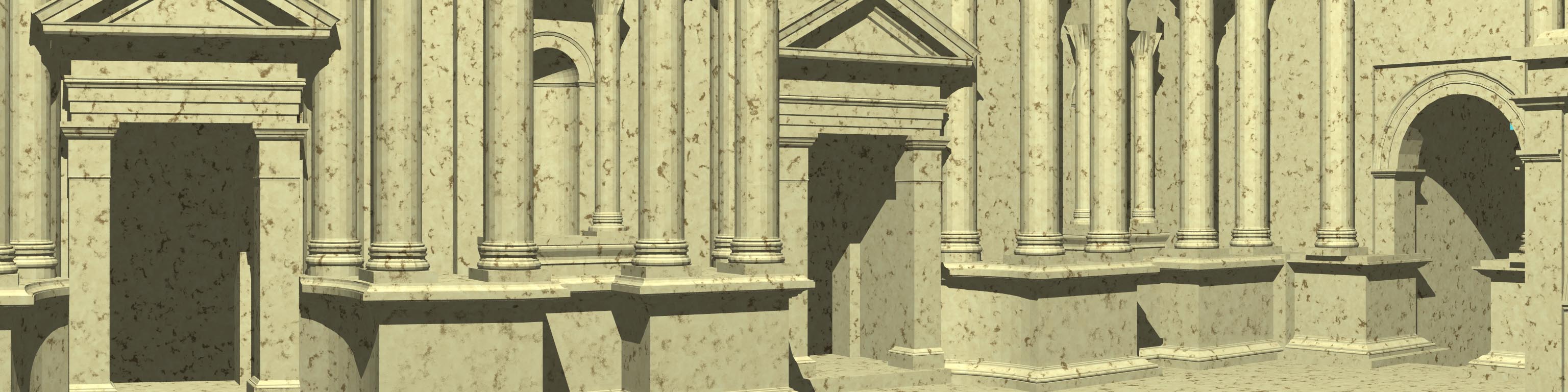
One thing to notice is the large variation in density of the polygons. A large number of polygons are used around the decorative parts of the columns and archways. 
It is quite straightforward to write an OpenGL viewer for this geometry. Since the geometry is static it can all be placed in a display list using
   glNewList(itemid,GL_COMPILE);
      :
   /* Draw the polygons here */
      :
   glEndList();
The camera is moved around controlled by the user, the scene is
rendered using
glCallList(itemid); With the OpenGL card available for this work the refresh rate was only about one frame per second, half that for viewing in stereo. The question then is what can be done to improve the frame rate. Certainly the biggest gains could be made by creating the geometry appropriately, for this exercise the geometry was taken as given. In many cases this is the situation, the software that created the model might not be available or the expertise/desire to make changes to a complicated model might not exist. 
A obvious saving for environments that one mainly wishes to walk inside is to only render the geometry that is in front of the camera, or even better, within the view frustum. (Which of these is chosen usually depends on the number of items that need to be tested against the view frustum, if large then the simpler in-front/behind test is faster.) In this case one obviously doesn't want to compare each facet at each time step. One solution is to subdivide the geometry into pieces, form a display list for each one but only draw those that are visible from the current camera position. 
The images here show the model subdivision at various levels of splitting. For a particular model there is an optimal level at which subdivision should be taken, too much and the intersection tests and display list handling dominate, too few and the geometry in the largest display list determines the frame rate. 
How the subdivision is done is by no means trivial. A couple of schemes were tried for this exercise, the one finally used was to decide on a number of subdivisions and iteratively bisect the subdivision containing the largest number of polygons. This tends to form subdivisions with approximately equal numbers of polygons, for example it can be seen that there are smaller subdivisions around the columns than the seats. A better algorithm would be to base the centers of the subdivisions on the dense areas within the geometry. It should also be noted that while in this case the subdivisions didn't overlap, that restriction could be lifted for a more efficient partitioning scheme.  Geometry Optimisation As well as doing things efficiently in OpenGL, there are some standard checks and transformations of the geometry that should be made whenever transforming geometry from a CAD package into an environment where "every polygon counts". There are a number of inefficiencies that can arise with modelling in a package such as AutoCAD and exporting the geometry through an intermediate format.
Multiwall and off-axis projectionWritten by Paul BourkeFebruary 2003
AutoCAD Model courtesy of Chris Little,
Stephanie Phan, Andrew Hutson,
The images shown here were created for a number of purposes: to illustrate the need for offaxis frustums for immersive environments, to test the movie playing performance of the recently released Matrox Parhelia 3 display cards, to demonstrate correct image creation and presentation at the CAEV (3 wall projection system at Melbourne University), and finally to test a more general camera specification in PovRay. The images below on the right illustrate the projection type. The red lines are the projection planes and the blue lines the border of the frustum. These are top views but the same offaxis frustum concept also applies vertically. For the correct or minimally distorted projection, the viewer should be located at the intersection of the blue lines. The key concept is that for correct projection the frustums change with the viewers position (requiring viewer head tracking) and the frustums are generally asymmetric All the images are 3072 by 768 and should therefore be a one to one match with projector pixels. All projections are based upon the screens being 2.4m wide and 1.8m high (4:3 ratio) with the side screens at an angle of 21 degrees (geometry of the test environment). It could be argued that the screens would be better angled at a greater angle than 21 degrees so as to bring the "sweet spot" (for 3 symmetric frustums, example 1) closer to the center of the room.
Multiple wall projectionUsing independent computers and OpenGL
December 2000 Introduction This document describes an approach to presenting 3 dimensional environments on multiple screens (projected onto large walls). The key challenges for this project included the following.
The hardware setup for this experiment was minimal, standard Linux (Intel based) boxes with GeForce OpenGL cards and 100MBit networking (10MBit was also shown to be satisfactory for the small communication volumes needed). While most testing was performed simply using three monitors placed in the right orientation, the system was operated in a couple of 2 and 3 wall installations with projectors creating a seamless wide angle image. 
Intermachine communication In order to ensure that the displays on each computer updated exactly in sync, a simple socket library was written using sock streams over TCPIP. (All the machine were on a 100MBit network). Note that even if all the computers were identical and updating as fast as they could, they wouldn't stay in synchronisation. The main source of variation occurs when the geometry complexity in one view is much greater than the other views. Since OpenGL does frustum culling, the complex views will render more slowly. 
The software was written with one machine acting as the server and all the others clients. The same binary served as both client and server. A few messages were defined that were exchanged between the clients and server, these could be extended for more complicated environments, for example, where the geometry was changing. The messages are briefly explained below.
So, the general flow is as follows. Whenever the user (controlling the server) chooses a menu item, that information is sent to the clients with the "flags" message. As the user drags the mouse controlling the camera position and orientation, the "vp" and "vd" messages are sent to the clients. Every 30ms the server tries to refresh its display, it sends the "update" message to each client and draws the geometry to its own back buffer. The server then waits for "ready" messages from each client, when everyone is ready the server sends a "swap" message at which point an essentially instantaneous buffer swap is performed on all machines. Performance
Strict performance tests haven't been performed because they rely on
so many factors (scene complexity and type, OpenGL hardware, machine
characteristics,....). For the particular configuration being used here,
for a scene with sufficient geometry that could only just render at
30fps on a single machine, introducing 3 synced machines incurred a penalty
of less than 2fps.
While no testing has yet been done on the performance/scaling for very
large numbers of walls, there was no further loss of frame rate for 5 walls.
OpenGL projection OpenGL is especially suited to this type of projection because it has a very general frustum functionality (glFrustum()) which allows one to create the so called "off-axis" projections needed. The standard perspective projection offered by most rendering engines is unsuitable because it assume the view position is along a line that is both normal to and passes through the center of the projection plane.  Wall configuration
The wall specification is totally general. So while all the example above show a 3 wall environment where all the walls are in line, in practice the tests were mostly performed on 3 walls where the two side walls are toed in by about 30 degrees. Another arrangement is shown below where the walls are arranged vertically. Another application for 2 synced machines is in passive stereographics where one machine handles the left eye and the other machine the right eye. This functionality was also used in the testing as well as a 5 wall environment.
Extensions
| ||||||||||||||||||||||||||||||||||||