Miscellaneous transformations and projectionsIn what follows are various transformations and projections, mostly as they apply to computer graphics.
See also:
Spherical Projections (Stereographic and Cylindrical)Written by Paul BourkeEEG data courtesy of Dr Per Line December 1996, Updated December 1999 StereographicThe stereographic projection is one way of projecting the points that lie on a spherical surface onto a plane. Such projections are commonly used in Earth and space mapping where the geometry is often inherently spherical and needs to be displayed on a flat surface such as paper or a computer display. Any attempt to map a sphere onto a plane requires distortion, stereographic projections are no exception and indeed it is not an ideal approach if minimal distortion is desired. A physical model of stereographic projections is to imagine a transparent sphere sitting on a plane. If we call the point at which the sphere touches the plane the south pole then we place a light source at the north pole. Each ray from the light passes through a point on the sphere and then strikes the plane, this is the stereographic projection of the point on the sphere. In order to derive the formulae for the projection of a point (x,y,z) lying on the sphere assume the sphere is centered at the origin and is of radius r. The plane is all the points z = -r, and the light source is at point (0,0,r). The cross section of this arrangement is shown below in what is commonly called a Schlegal diagram. 
Consider the equation of the line from P1 = (0,0,r) through a point
P2 = (x,y,z) on the sphere,
Solving this for mu for the z component yields or This is then substituted into (1) to obtain the projection of any point (x,y,z) Note
The following example is taken from the mapping of EEG data recorded on an approximate hemisphere (human head). The data can be rendered on a virtual hemisphere but as such the whole field is not readily visible from any particular viewpoint. The best option is to view the data from the top of the head but the effects around the rim are hard to interpret due to the compression of information as a result of the curvature of the surface. 
The following shows a planar projection from the hemisphere on the left and the same data with a stereographic projection. The compression near the rim is clearly reduced greatly improving the visibility of the results in that region. 
Note that in the above, after the projection has been performed, the resulting disk is scaled by a factor of 0.5 in order to retain the same dimensions as the hemisphere. Cylindrical projectionAlso sometimes known as a cylindric projection.
The general cylindrical projection is one where lines of latitude are projected to equally spaced parallel lines and lines of longitude are projected onto not necessarily equally spaced parallel lines. The diagram below illustrates the basic projection, a line is projected from the centre of the sphere through each point on the sphere until it intersects the cylinder. 
The equations are quite straightforward, if the cylinder is unwrapped and the horizontal axis is x and the vertical axis is y (origin in the vertical center and on the left side horizontally) then: y = constant * tan(beta)
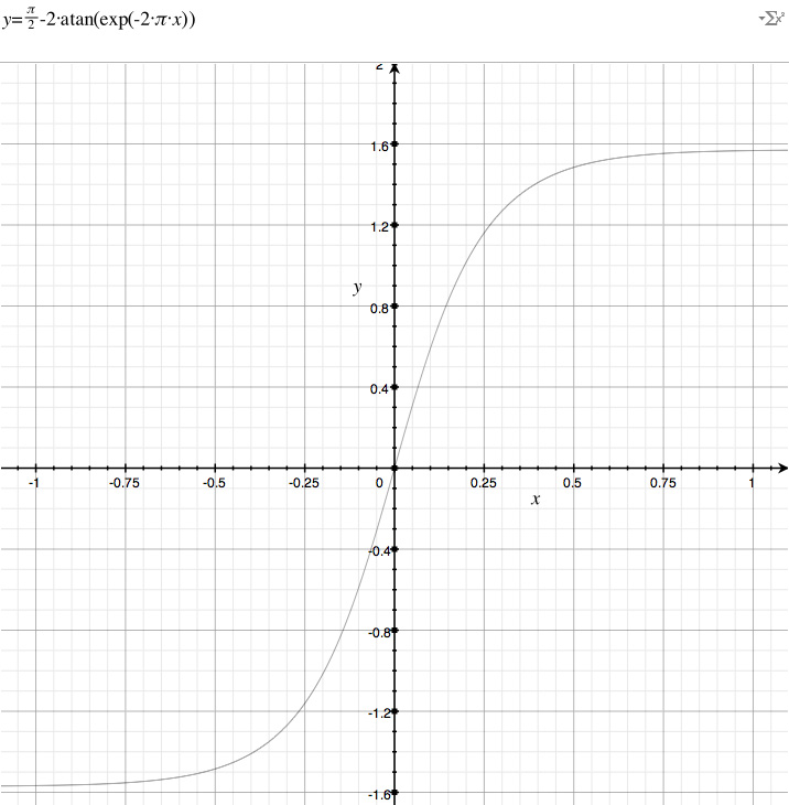
Mercator projectionA Mercator projection is similar in appearance to a cylindrical projection but has a different distortion in the spacing of the lines of longitude. Like the cylindrical projection north and south are always vertical and east and west are always horizontal. Also it cannot represent the poles because the mathematics have an infinity singularity there. This is one of the more common projections used in mapping the Earth onto a flat surface. There is not a single Mercator projection because one can choose the maximum value for the latitudes, a common convention is illustrated below.
The equations for longitude and latitude in terms of normalised image coordinates (x,y) (-1..1) are as follows. latitude = atan(exp(-2 * pi * y))
The reverse mapping is y = ln((1 + sin(latitude))/(1 - sin(latitude))) / (4 pi)
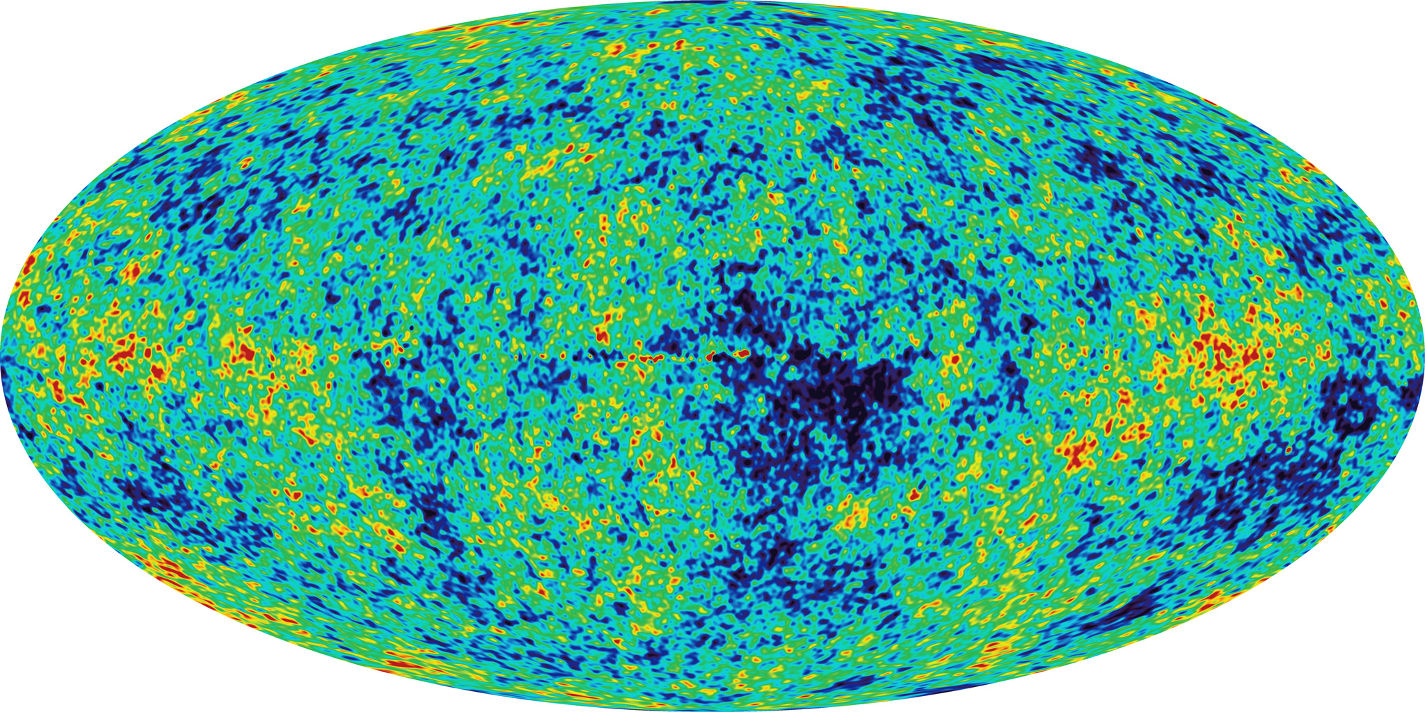
Cylindrical projections in general have an increased vertical stretching as one moves towards either of the poles. Indeed, the poles themselves can't be represented (except at infinity). This stretching is reduced in the >Mercator projection by the natural logarithm scaling. Direct Polar, known as Spherical or Equirectangular ProjectionWhile not strictly a projection, a common way of representing spherical surfaces in a rectangular form is to simply use the polar angles directly as the horizontal and vertical coordinates. Since longitude varies over 2 pi and latitude only over pi, such polar maps are normally presented in a 2:1 ratio of width to height. The most noticeable distortion in these maps is the horizontal stretching that occurs as one approaches the poles from the equator, this culminates in the poles (a single point) being stretched to the whole width of the map. An example of such a map is given below for the Earth.

While such maps are rarely used in cartography, they are very popular in computer graphics since it is the standard way of texture mapping a sphere.....hence the popularity of maps of the Earth as shown above.
Hammer-Aitoff map projectionConversion to/from longitude/latitudeWritten by Paul BourkeApril 2005 An Aitoff map projection (attributed to David Aitoff circa 1889) is a class of azimuthal projection, basically an azimuthal equidistant projection where the longitude values are doubled (squeezing 2pi into pi) and the resulting 2D map is stretched in the horizontal axis to form a 2:1 ellipse. In a normal azimuthal projection all distances are preserved from the tangent plane point, this is not the case for a Aitoff projection, except along the vertical and horizontal axis. A modification to the Aitoff projection is the Hammer-Aitoff projection which has the property of preserving equal area over the whole map. Conversion from longitude/latitude to Hammer-Aitoff coordinates (x,y)Consider longitude to range between -pi and pi, latitude between -pi/2 and pi/2.
(x,y) are each normalised coordinates, -1 to 1. Conversion of Hammer-Aitoff coordinates to longitude/latitude
The Hammer-Aitoff map is limited to where (x longitude) >= 0.
Example: Conversion of longitude/latitude to Hammer-Aitoff coordinates
Example: Conversion of Hammer-Aitoff coordinates to longitude/latitude
Transformations on the planeWritten by Paul BourkeJanuary 1987 The following describes the 2d transformation of a point on a plane P = ( x , y ) -> P' = ( x' , y' )
TranslationA translation (shift) by Tx in the x direction and Ty in the y direction is
x' = x + Tx
ScalingA scaling by Sx in the x direction and Sy in the y directions about the origin is
x' = Sx x
If Sx and Sy are not equal this results in
a stretching along the axis of the larger scale factor.
x' = x0 + Sx ( x - x0 )
RotationRotation about the origin by an angle A in a clockwise direction is
x' = x cos(A) + y sin(A) To rotate about a particular point apply the same technique as described for scaling, translate the coordinate system to the origin, rotate, and the translate back. ReflectionReflection about the x axis
x' = x Reflection about the y axis
x' = - x Reflections about an arbitrary line involve possibly a translation so that a point on the line passes through the origin, a rotation of the line to align it with one of the axis, a reflection, inverse rotation and inverse translation. ShearA shear by SHx in the x axis is accomplished with
x' = SHx x A shear by SHy in the y axis is accomplished with
x' = x
Coordinate System TransformationWritten by Paul BourkeJune 1996 There are three prevalent coordinate systems for describing geometry in 3 space, Cartesian, cylindrical, and spherical (polar). They all provide a way of uniquely defining any point in 3D.
The following illustrates the three systems.
Equations for converting between Cartesian and cylindrical coordinates 
Equations for converting between cylindrical and spherical coordinates 
Equations for converting between Cartesian and spherical coordinates 
Rotations about each axis are often used to transform between different coordinate systems, for example, to direct the virtual camera in a flight simulator. These angles often go by different names, in the discussion here I will use a right hand coordinate system (y "forward", x to the right, and z upwards). As such rotation about the z axis will be referred to as direction, rotation about the y axis is roll (sometimes called bank), and rotation about the x axis is pitch. Further, a rotation will be considered positive if it is clockwise when looking down the axis towards the origin. Other conventions will be left as an exercise for the reader. The three rotation matrices are given below, note that they seem asymmetric with respect to the sign of the sin() term.
Rotation by tx about the x axis
Rotation by ty about the y axis
Rotation angle tz about the z axis
A characteristic of applying these transformations is that the order is important. If the rotation matrices above are called Rx(t), Ry(t), and Rz(t) respectively then applying the rotations in the order Rz(t) Rx(t) Ry(t) will in general result in a different result to another order, say Rx(t) Ry(t) Rz(t). In what follows a particular order will be discussed and the other combinations will be left up to the reader to derive based on the same approach. The particular order of rotations applied here is to rotate about the y axis first (roll), they the x axis (pitch), then the z axis (direction). This is perhaps the most common order is usage in games and flight simulators.
The single (combined) matrix is
One other requirement is given a new coordinate system how does one derive the corresponding three Euler angles. If the orthonormal vectors of the new coordinate system are X,Y,Z then the transformation matrix from (1,0,0), (0,1,0), (0,0,1) to the new coordinate system is
so
Also so
And lastly so Note:
Converting between left and right hand coordinate systemsWritten by Paul BourkeMay 2001
Computer based modelling and rendering software seem to be split evenly between whether they use a left hand or right hand coordinate system, for example OpenGL uses a right hand system and PovRay a left hand system. This document describes bow to convert model coordinates and/or camera attributes when transferring models from one package to another. Each system is shown below, the difference involves how the cross product is defined...using the so-called left or right hand rule.  Note that the exact orientation of the axes above is not relevant, y need not be "pointing up", z need not be pointing "into the page". All axes orientations are equivalent to one of the above after a suitable rotation. There are two ways to convert models between systems so that the rendered results are identical. The first involves inverting the x value (any single axes will do) of all vertices in the model and camera settings, the second uses the model and camera coordinates without change but requires a flipping of any rendered image horizontally. In what follows, the symbols p, d, and u will represent the vectors position, view direction, and up vector respectively. Method 1 - inverting the x coordinates
Method 2 - flipping image horizontally In this case the coordinates of the model and camera are used unchanged when transferring from one system to the other. As can be seen in the example below, the image ends up being horizontally flipped.  This is usually the preferred method, perhaps mainly because it avoids worrying about which system one is using until the end of the process, the image flipping can be built into post processing image tools. Also, it means that if one makes a mistake regarding which system is being using it doesn't affect the rendered result nearly as seriously than if one got made a mistake in the first method. You may wonder why it is the horizontal axis that is flipped, what is so special about it? That arises because the flip is actually about the up vector which is traditionally vertical on the rendered image.
Classification of 3D to 2D projectionsWritten by Paul BourkeDecember 1994 The following classifies the most common projections used to represent 3D geometry on a 2D surface. Each projection type has a brief comment describing its unique characteristic. 
Oblique projections
Note:
Correction of Planar (Stretch) DistortionWritten by Paul BourkeNovember 1989 The following mathematics and illustrations came from a project to undistort photographs taken of a flat piece of land. The photographs were taken from various angles to the ground and thus needed to be "straightened" so that relative area measures could be taken. The same technique could of course be used to intentionally distort rectangular areas. The conventional (Cartesian) method of uniquely specifying a point in 2 dimensions is by two coordinates. For the unit square below these two coordinates will be called mu and delta, they are the relative distances along the horizontal and vertical edges of the square. 
If the square above is linearly distorted (stretched) the internal coordinate mesh is also distorted but the relative distances (mu and delta) of a point P along two connected edges remains the same. 
To undistort any point P within the polygon we need to find the ratios mu and delta. Point A is given by:  Point B is given by
 For the point P along the line AB
 Substituting for A and B, equation 1

This gives two equations, one for the x coordinate and the other for the y coordinate, equation 2,3 
Dividing equation (2) by (3) removes delta, solving for mu gives a quadratic of the form  where
 After solving the quadratic for mu, delta can be calculated from (1) above.
Each of the different distortions will be illustrated by using the following simple diagram. 
For the following examples an additional grid will be placed over the image to further illustrate the nature of the distortion. Each type of distortion has controls associated with it, these are indicated by black "blobs" at the current position of the control points. To vary these parameters simply click and drag the control points.
Mappings in the Complex PlaneWritten by Paul BourkeJuly 1997 The following illustrates the general form of various mappings in the complex plane. The mappings are applied to part of a unit disk centered at the origin as shown on the left hand side. The circle is filled with rays from the origin and arcs centered about the origin. A series of coloured rays further illustrate the mapping orientation.
World to Screen Projection TransformationWritten by Paul BourkeDecember 1994 The representation by computer of 3 dimensional forms is normally restricted to the projection onto a plane, namely the 2 dimensional computer screen or hard copy device. The following is a procedure that transforms points in 3 dimensional space to screen coordinates given a particular coordinate system, camera and projection plane models. This discussion describes the mathematics required for a perspective projection including clipping to the projection pyramid with a front and back cutting plane. It assumes the projection plane to be perpendicular to the view direction vector and thus it does not allow for oblique projections. Included in the appendices is source code (written in the C programming language) implementing all the processes described. Coordinate systemIn what follows a so called right handed coordinate system is used, it has the positive x axis to the right, the positive z axis upward, and the positive y axis forward (into the screen or page). Conversion between this and other coordinate systems simply involves the swapping and/or negation of the appropriate coordinates. Camera modelThe camera is fundamentally defined by its position (from), a point along the positive view direction vector (to), a vector defining "up" (up), and a horizontal and vertical aperture (angleh, anglev).
These parameters are illustrated in the following figure.
One obvious restriction is that the view direction must not be collinear with the up vector. In practical implementations, including the one given in the appendices, the up vector need not be a unit vector. Other somewhat artificial variables in the camera model used here are front and back clipping planes, a perspective/oblique projection flag, and a multiplicative zoom factor. The clipping planes are defined as positive distances along the view direction vector, in other words they are perpendicular to the view direction vector. As expected all geometry before the front plane and beyond the back plane is not visible. All geometry which crosses these planes is clipped to the appropriate plane. Thus geometry visible to a camera as described here lies within a truncated pyramid.
Screen model The projection plane (computer screen or hard copy device) can be defined in many ways. Here the central point, width and height are used. The following will further assume the unfortunate convention, common in computer graphics practice, that the positive vertical axis is downward. The coordinates of the projection space will be referred to as (h,v). Note that normally in computer windowing systems the window area is defined as an rectangle between two points (left,top) and (right,bottom). Transforming this description into the definition used here is trivial, namely horizontal center = (left + right) / 2vertical center = (top + bottom) / 2 width = right - left height = bottom - top
The units need not be specified although they are generally pixel's, it is assumed that there are drawing routines in the same units. It is also assumed that the computer screen has a 1:1 aspect ratio, a least as far as the drawing routines are concerned. A relationship could be made between the ratio of the horizontal and vertical camera aperture and the horizontal and vertical ratio of the display area. Here it will be assumed that the display area (eg: window) has the same proportions as the ratio of the camera aperture. In practice this simply means that when the camera aperture is modified, the window size is also modified so as to retain the correct proportions. AlgorithmThe procedure for determining where a 3D point in world coordinates would appear on the screen is as follows:
Transforming a line segment involves determining which piece, if any, of the
line segment intersects the view volume. The logic is shown below.
Clipping Two separate clipping processes occur. The first is clipping to the front and back clipping planes and is done after transforming to eye coordinates. The second is clipping to the view pyramid and is performed after transforming to normalised coordinates at which point it is necessary to clip 2D line segments to a square centered at the origin of length and height of 2.
Source code
Triangle coordinatesWritten by Paul BourkeSeptember 2020 In the following a point P is decomposed into two components, ua and u2. The following shows the conventions and symbols used here. 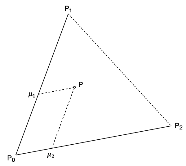
If the system is translated to place P0 at the origin then the point P in question can be written as.
In matrix form. 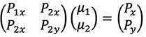
Which is solved as. 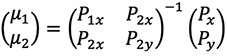
Which expands as follows. 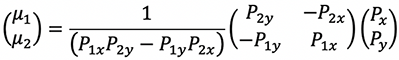
Mapping from box to warped boxWritten by Paul BourkeDecember 2020 The following illustrates the (simple) maths for mapping a point in a box (axis aligned) into a warped box. The warped box is defined by the values of the 8 vertices, noting that the vertices of each face need to be coplanar. The following applies the x cut first then y and finally z. But the cuts can be made in any order with the same result. 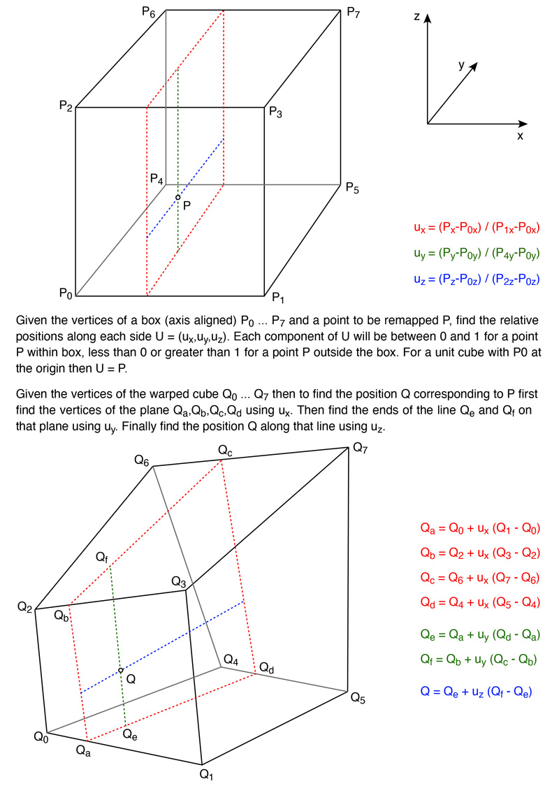
While the above is normally used to warp points within the original box, the maths applies perfectly well for points outside the box, as if the warped box also distorts the whole of space. Points within the box have ux, uy and uz in the range of 0 to 1. Values outside this range correspond to points outside the box. |