Tiling Textures on the Plane (Part 1)Written by Paul BourkeSeptember 1992
In many texturing applications it is necessary to be able to "tile" the texture over a larger region than the texture segment covers. In the ideal case the texture segment automatically tiles, that is, if it laid out in a grid it forms a seamless appearance. For example consider the following texture.  
Many textures of tiles form such seamless surfaces easily because they are naturally bounded by rectangular discontinuities. For example consider the tile  Laid out it forms the tiling below  Other regular tiles fit together in more subtle ways.   For texture segments that don't have strong directional structure a common tiling method involves mirroring each second segment so that adjacent edges match, this is illustrated below 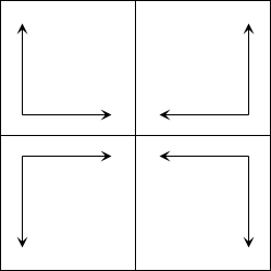 and here in a real example 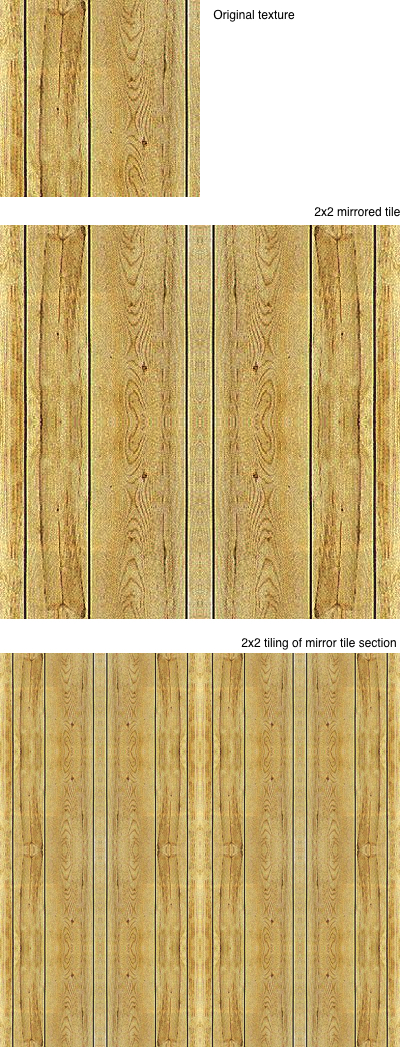
This larger segment can now be repeated in the normal way indefinitely as all the edges will now join without discontinuities. Sometimes a mixture of mirroring and direct tiling can be applied, that is, mirror tile in one direction and do a straightforward tile in the other direction. In what follows one method will be discussed for making any image tile with reduced seams. In the following the image on the left will be used as an example, it clearly doesn't tile. The discontinuities between the tiles can be illustrated by swapping the diagonal halves of the image as shown on the right. Sometimes it is possible to edit the image on the right, smoothing out the center vertical and horizontal seams, the result would then tile. In general this is difficult and has the disadvantage of being a manual process.
In what follows, let the original image be represented as O, for simplicity consider the image to be square with N pixels vertically and horizontally. Each pixel is indexed (C conventions) as O[i][j] where i and j range from 0 to N-1. The diagonally swapped image will be referred to as Od. Each pixel in Od is found as follows (assuming N is even):
Two masks are created, there are many alternatives but the example shown below is a radial linear ramp from black to white. Other masks can be used, the requirement is that the mask tends smoothly to pure white at the image boundary. The second mask on the right is diagonal swapped version of the mask on the left.
The mask shall be referred to as M. The mask above can be formed by the following: Where i and j range from 0 to N/2-1. Md is calculated as for Od above.
The following two images are created by multiplying the two original images by their respective masks. I've chosen a slightly different convention here to normal, here for purposes of the multiplication black has a value of 1 and white 0. These two images tile (although rather boringly) because the left image decays to zero at it's edges.
And finally, the tilable image on the left is created by averaging the two images above. On the right is a reduced 2x2 tiling of the tile on the left showing the absence of any discontinuities.
If T is the tilable texture, this can be written as
Note that to avoid zero divide by the denominators above it is customary constrain the mask values to positive (non zero) values.
This linear mask is calculated as follows:
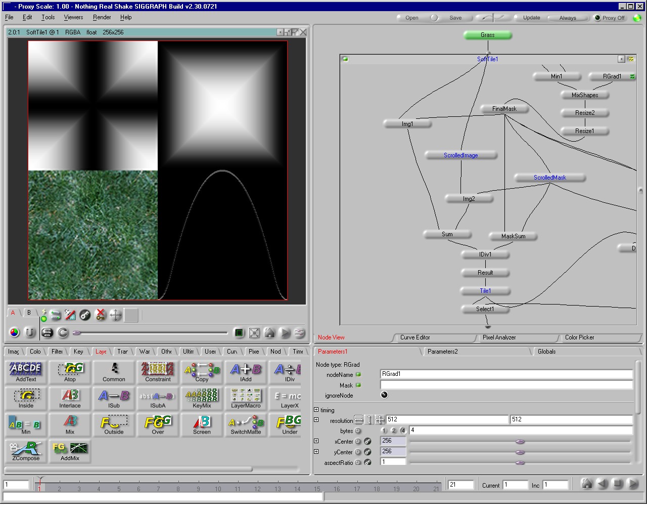
For perhaps a more realistic texture, consider the following photograph of some grass.
A detailed leaf example.
Software
Parametric Equation of a Sphere and Texture MappingWritten by Paul BourkeAugust 1996 One possible parameterisation of the sphere will be discussed along with the transformation required to texture map a sphere. An angle parameterisation of the sphere is
y = r sin(theta) sin(phi) z = r cos(theta) where r is the radius, theta the angle from the z axis (0 <= theta <= pi), and phi the angle from the x axis (0 <= phi <= 2pi). Textures are conventionally specified as rectangular images which are most easily parameterised by two cartesian type coordinates (u,v) say, where 0 <= u,v <= 1. The equation above for the sphere can be rewritten in terms of u and v as
y = r sin(v pi) sin(u 2 pi) z = r cos(v pi) Solving for the u and v from the above gives
u = ( arccos(x/(r sin(v pi))) ) / (2 pi) So, given a point (x,y,z) on the surface of the sphere the above gives the point (u,v) each component of which can be appropriately scaled to index into a texture image. Note
#define PI 3.141592654
#define TWOPI 6.283185308

void SphereMap(x,y,z,radius,u,v)
double x,y,z,r,*u,*v;
{
   *v = acos(z/radius) / PI;
   if (y >= 0)
      *u = acos(x/(radius * sin(PI*(*v)))) / TWOPI;
   else
      *u = (PI + acos(x/(radius * sin(PI*(*v))))) / TWOPI;
}
There are still two special points, the exact north and south poles of the sphere, each of these two points needs to be "spread" out along the whole edge v=0 and v=1. In the formula above this is where sin(v pi) = 0.
OpenGL sphere with texture coordinatesWritten by Paul BourkeJanuary 1999 A more efficient contribution by Federico Dosil: sphere.c While straightforward many people seem to have trouble creating a sphere with texture coordinates. Here's the way I do it (written for clarity rather than efficiency). 
Note
/*
   Create a sphere centered at c, with radius r, and precision n
   Draw a point for zero radius spheres
*/
void CreateSphere(XYZ c,double r,int n)
{
   int i,j;
   double theta1,theta2,theta3;
   XYZ e,p;

   if (r < 0)
      r = -r;
   if (n < 0)
      n = -n;
   if (n < 4 || r <= 0) {
      glBegin(GL_POINTS);
      glVertex3f(c.x,c.y,c.z);
      glEnd();
      return;
   }

   for (j=0;j<n/2;j++) {
      theta1 = j * TWOPI / n - PID2;
      theta2 = (j + 1) * TWOPI / n - PID2;

      glBegin(GL_QUAD_STRIP);
      for (i=0;i<=n;i++) {
         theta3 = i * TWOPI / n;

         e.x = cos(theta2) * cos(theta3);
         e.y = sin(theta2);
         e.z = cos(theta2) * sin(theta3);
         p.x = c.x + r * e.x;
         p.y = c.y + r * e.y;
         p.z = c.z + r * e.z;

         glNormal3f(e.x,e.y,e.z);
         glTexCoord2f(i/(double)n,2*(j+1)/(double)n);
         glVertex3f(p.x,p.y,p.z);

         e.x = cos(theta1) * cos(theta3);
         e.y = sin(theta1);
         e.z = cos(theta1) * sin(theta3);
         p.x = c.x + r * e.x;
         p.y = c.y + r * e.y;
         p.z = c.z + r * e.z;

         glNormal3f(e.x,e.y,e.z);
         glTexCoord2f(i/(double)n,2*j/(double)n);
         glVertex3f(p.x,p.y,p.z);
      }
      glEnd();
   }
}
It is a small modification to enable one to create subsets of a sphere....3 dimensional wedges. As an example see the following code.
/*
   Create a sphere centered at c, with radius r, and precision n
   Draw a point for zero radius spheres
   Use CCW facet ordering
   "method" is 0 for quads, 1 for triangles
      (quads look nicer in wireframe mode)
   Partial spheres can be created using theta1->theta2, phi1->phi2
   in radians 0 < theta < 2pi, -pi/2 < phi < pi/2
*/
void CreateSphere(XYZ c,double r,int n,int method,
   double theta1,double theta2,double phi1,double phi2)
{
   int i,j;
   double t1,t2,t3;
   XYZ e,p;

   /* Handle special cases */
   if (r < 0)
      r = -r;
   if (n < 0)
      n = -n;
   if (n < 4 || r <= 0) {
      glBegin(GL_POINTS);
      glVertex3f(c.x,c.y,c.z);
      glEnd();
      return;
   }

   for (j=0;j<n/2;j++) {
      t1 = phi1 + j * (phi2 - phi1) / (n/2);
      t2 = phi1 + (j + 1) * (phi2 - phi1) / (n/2);

      if (method == 0)
         glBegin(GL_QUAD_STRIP);
      else
         glBegin(GL_TRIANGLE_STRIP);

      for (i=0;i<=n;i++) {
         t3 = theta1 + i * (theta2 - theta1) / n;

         e.x = cos(t1) * cos(t3);
         e.y = sin(t1);
         e.z = cos(t1) * sin(t3);
         p.x = c.x + r * e.x;
         p.y = c.y + r * e.y;
         p.z = c.z + r * e.z;
         glNormal3f(e.x,e.y,e.z);
         glTexCoord2f(i/(double)n,2*j/(double)n);
         glVertex3f(p.x,p.y,p.z);

         e.x = cos(t2) * cos(t3);
         e.y = sin(t2);
         e.z = cos(t2) * sin(t3);
         p.x = c.x + r * e.x;
         p.y = c.y + r * e.y;
         p.z = c.z + r * e.z;
         glNormal3f(e.x,e.y,e.z);
         glTexCoord2f(i/(double)n,2*(j+1)/(double)n);
         glVertex3f(p.x,p.y,p.z);

      }
      glEnd();
   }
}
Texture map correction for spherical mappingWritten by Paul BourkeJanuary 2001
Lua/gluas script contributed by Philip Staiger. When texture mapping a sphere with a rectangular texture image with polar texture coordinates, the parts of the image near the poles get distorted. Given the different topology between a sphere and plane, there will always be some nonlinear distortion or cut involved. This normally manifests itself in pinching at the poles where rows of pixels are being compressed tighter and tighter together the closer one gets to the pole. At the poles is the extreme case where the whole top and bottom row of pixels in the texture map is compressed down to one point. The spherical images below on the left are examples of this pinching using the rectangular texture also on the left.
It is simple to correct for this by distorting the texture map. Assume the texture map is mapped vertically onto lines of latitude (theta) and mapped horizontally onto lines of longitude (phi). There is no need to modify theta but phi is scaled as we approach the two poles by cos(theta). The diagram below illustrates the conventions used here.
The pseudo-code for this distortion might be something like the following, note that the details of how to create and read the images are left up to your personal preferences.
   double theta,phi,phi2;
   int i,i2,j;
   BITMAP *imagein,*imageout;

   Form the input and output image arrays
   Read an input image from a file

   for (j=0;j<image.height;j++) {
      theta = PI * (j - (image.height-1)/2.0) / (double)(image.height-1);
      for (i=0;i<image.width;i++) {
         phi  = TWOPI * (i - image.width/2.0) / (double)image.width;
         phi2 = phi * cos(theta);
         i2  = phi2 * image.width / TWOPI + image.width/2;
         if (i2 < 0 || i2 > image.width-1) {
            newpixel = red;                         /* Should not happen */
         } else {
            newpixel = imagein[j*image.width+i2];
         }
         imageout[j*image.width+i] = image.newpixel;
      }
   }

   Do something with the output image
Applying this transformation to a regular grid is show below.
Perhaps a more illustrative example is given below for a "moon" texture. Note that in general if the texture tiles vertically and horizontally then after this distortion it will no longer tile horizontally. A number of tiling methods can be used to correct for this. One is to replicate and mirror the texture horizontally, since the distortion is symmetric about the horizontal center line of the image, the result will tile horizontally. Another method is to overlap two copies of the texture after the distortion with appropriate masks that fade the appropriate texture out at the non-tiling borders.
This final example illustrates how after the distortion the image detail is evenly spread over the spherical object instead of acting like lines of longitude that get closer near the poles.
Texture mapping a fisheye projection onto a hemisphereWritten by Paul BourkeApril 2012 The following illustrates how to calculate the texture coordinates for the vertices of a hemisphere such that a fisheye image can be applied as a texture with the "expected" results. To test the mathematics and code presented here the following texture image will be used, the expected result is for the hemisphere to be textured with lines of longitude and latitude. 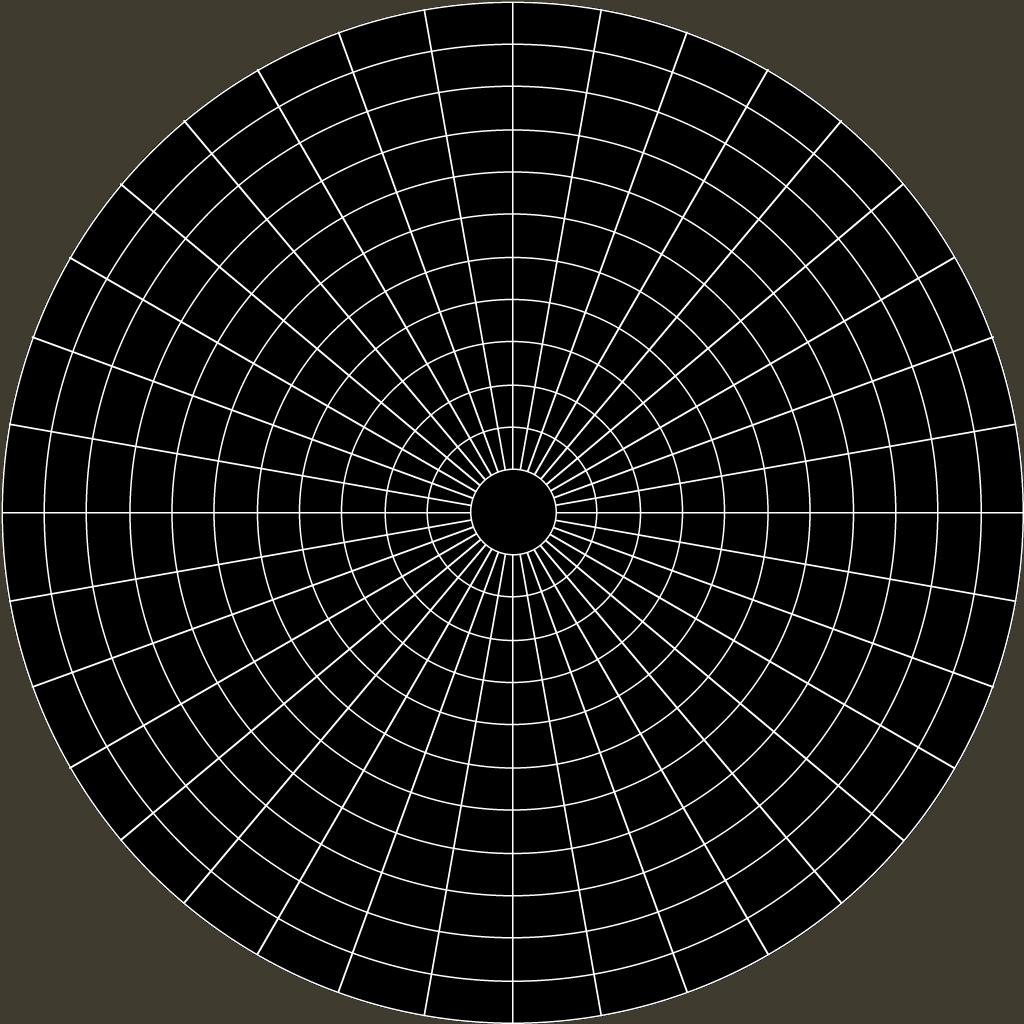
The texture coordinate for any vertex of the hemisphere mesh is calculated by determining the polar angles theta and phi. These can then be mapped directly into the fisheye texture plane. The equations are shown below and also in the source code provided. 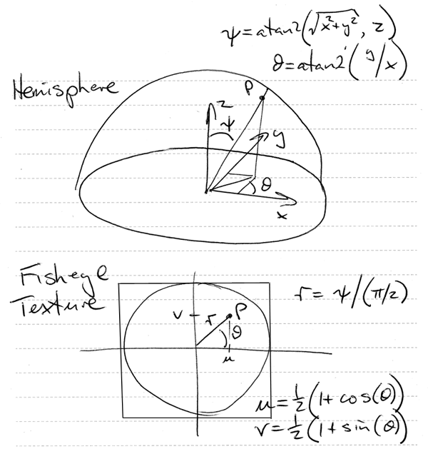
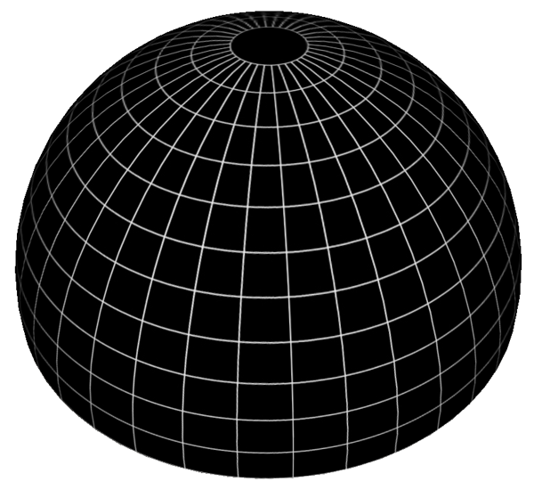
Source code that illustrates this is give here (tab stops set to 3 for correct indenting): fishtexture.c. It creates a textured hemisphere centered at the origin with unit radius described as an obj file: fishtexture.obj with associated material file: fishtexture.mtl. Resulting views of the above obj file. 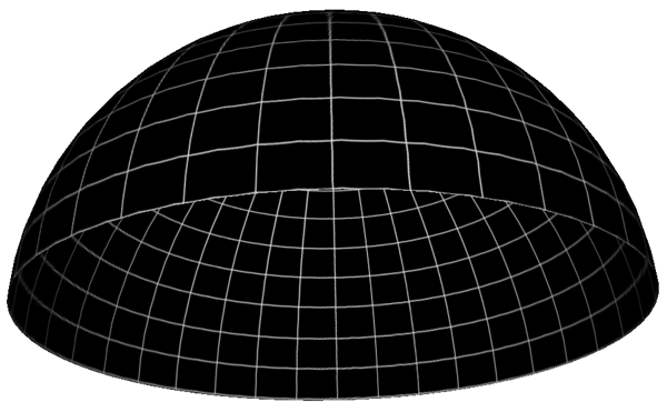
Texture Mapping Schemes in Common UsageWritten by Paul BourkeMarch 1987
Planar
Cubic
Cylindrical
Rectangular Cylindrical
Spherical
Miscellaneous examples
|


