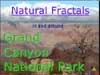
Natural Fractals in Grand Canyon National ParkBy Gayla ChandlerIntroduction
I gave this presentation as a special program at Grand Canyon National Park in the Shrine
of the Ages on Friday 31 December 2004 and Saturday 1 January 2005. The slide show
and notes are now accessible from the web for viewing by individuals and/or use by teachers in classrooms. What I
ask in return is that no changes be made to the materials. Suggestions will be
appreciated and changes made if deemed appropriate.
Using the slides as slates for your own markings by highlighting similarity in the images may provide a richer viewing experience. (Instructions for doing this in PowerPoint are available on every slide.) Let this be an active experience. Play with it. The marks are only there while the slide is up. Every slide is shown below in thumbnail form with its respective notes. The thumbnails have very low resolution. The images in the presentation, however, have fairly good resolution, hopefully they will be projector quality (set the projector for 800x600 image size).
Download 
"Natural Fractals" is hyperlinked to the Earth Monitoring System website's Nonlinear Geoscience Fractals page. This site provides easy to read information about fractal systems in nature, focusing on geology. I think it is an appropriate introductory link for a presentation about natural fractals in the Grand Canyon! It is a friendly site to explore. The link was originally to the main page of the Yale Fractal Geometry website, the most comprehensive web source that I know of for technical information about fractals. Many links to Yale's pages are scattered throughout the presentation, plus, the Snow section is taken verbatim from their site.
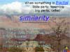
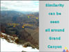
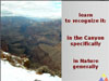
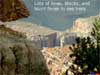
Although all images in this presentation were taken at Grand Canyon, the presentation focuses on similarity in nature generally, i.e., not just at Grand Canyon. I often use the term similarity instead of self-similarity. Natural fractals have self-similar properties. Keep in mind, however, that the exact self-similarity in geometric fractals and the approximate self-similarity in natural fractals are not identical. Even though not identical, they share significant properties that include scale-invariance and similar shapes that repeat on different scales. The first link on this slide is terrific for kids. It goes to Cynthia Lanius main fractals page. If you use the search term fractals in Google, Cynthia's page is the first hit, it is the number one fractals page, is very friendly and upbeat is geared toward children and the information presented is credible. The second link is to Paul Bourke's Self Similarity page. Paul's site is diverse in content, and is technologically advanced. It is a high-end site geared toward adults. It has to be one of the most fun sites to explore, if you like math and the sciences. On this page, he does a great job of showing similarity on different scales, and scale-invariance (aka scale independence). This is a fine page for beginners to the subject from both a words and visual standpoint. What shape the parts are depends entirely on the object. This cannot be overstated. Let me breeze ahead to Slide 56 in the presentation, the first slide where a Sierpinski tetrahedron is sitting in an image. If you see a Sierpinski tetrahedron in one of my pictures, it doesn't imply that nature is filled with triangles and/or tetrahedra or any like thing. Repeated experiences around people while out taking photographs with the structures over the past three years have shown me that this is a common assumption to jump to, and, once jumped to it is very hard for people adults and children alike to undo. Nature has its own shapes that are typically completely different from familiar shapes in Euclidean geometry, although we will see some intersections of nature with Euclidean shapes in the Canyon section. In the Canyon, we will be looking for shapes like lines and boxes, blocks, and rectangles. The Canyon has a lot of rectilinear structure.
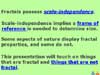
This slide provides links to information about scale-invariance, the magnification symmetry of fractals, connections between fractals and chaos, and some perspective about what is fractal and what is not. Usually when we're walking around, there are objects around to indicate how big something is. We can see a lot of scaling in tree limbs, for instance, several stages of substructure are present. Tree limbs are scale-invariant even when there is no question about the size of the limbs. The point is that if there were no frame of reference, a tiny section of tree could be magnified and passed off as a bigger section: symmetry of magnification. The EMS page gives a good description of chaotic processes. One example of things fractal but not chaotic: geometric fractals because they are completely deterministic. There is nothing uncertain about the way they are going to grow or the shape they will become at infinity. An example of something chaotic but not fractal: frenzied ocean waves, and highly turbulent water generally. Apparently, similar substructure isn't present once a certain level of turbulence is reached when the process gets too wild, randomness may completely take over (I'm only trying to give a sense of the situation, am not speaking with authority about this). I have also included a link to Yale's page about "things that look like fractals but aren't", to reinforce that everything isn't fractal, and to give a sense about what is fractal and what is not. Now, some of the examples on the page don't connect with me personally, I would prefer some examples that are more concrete, but hopefully the page will add some perspective to your experience.
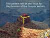
This slide provides valuable information about the presentation, and should be read. The topic slides follow. On slides 5-11, the topic introduced will be underlined, which signifies a link. Several of these links go to pages with artificial counterparts to the real world systems addressed in the topics.
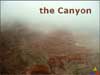
The Canyon , meaning the Canyon itself, is the longest section of the presentation. The link will take you to Paul Bourke's main page for fractal terrains. Right underneath the Canyon link is a another link to a page Paul wrote about how to make a fractal landscape. The Grand Canyon has a fractal dimension of ~2.25.
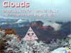
The topic introduced is Clouds, with a link to a url that gives different perspectives about them. One of the sections in the link is entitled: Clouds are not fractal and makes the point that although fractal geometry describes certain aspects of clouds (including complexity, and general shape), there are many aspects of clouds and cloud behaviour that fractal geometry doesn't explain at all.
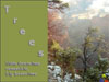
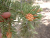
Trees are the topic. The link goes to a site with some fractal trees and bushes. The branches in trees and bushes are almost always fractal, whereas their outer foliage rarely is. There is good reason for this, referenced in slides 78 and 86.
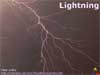
Lightning. The link goes to a Yale Fractal Geometry page with a series of pictures of natural fractals, one of which is lightning.
"Boundaries" links to a set of fractal games from an NSF-funded program that I attended for several summers out of Florida Atlantic University (FAU) in Boca Raton. "Coastlines" is the fractal boundaries game. It is very easy to play, and it is fun to change the parameters to arrive at different coastline appearances. IMPORTANT NOTE: these games were created using Java language. Windows no longer comes with the ability to run Java. If your computer is fairly new, you might have to download the necessary software to run these games and other Java programs, available at no charge, at: http://java.sun.com. I am told it is a fairly time-consuming download.
Rocks. I have linked to some general information about geology and fractals. It is good from a perspective standpoint and fits in well with my presentation. I disagree with one thing said on the page. It is stated that the detail in (natural) fractals goes on ad infinitum. In nature, however, this really isn't the case. Greater detail that goes on forever is the idea behind fractals, yes, but in nature this idea can t play out all the way. For instance, you can t keep breaking a rock into smaller rocks, forever, eg., the fractal structure of a natural object doesn't go all the way to its atomic structure. Whatever the specific similarity aspect you are observing in a natural object, that object will have pre-fractal states where the shape-similarity aspect is not present.
Snowflakes. This link takes you to Kenneth Libbrecht's snowflake site with all-real snowflake images taken with a special photo microscope. Libbrecht also makes snowflakes using an electric needle of some sort. It is a fabulous site to explore. His focus is not on fractals, you won t hear him even say the word fractal, even though he says much of the same things. The section on snow in my presentation, however it is taken verbatim from the Yale Fractal Geometry website is presented from a fractals perspective and uses all the proper lingo. I have included a link to the Yale Snow page on slide 120.
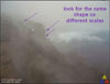
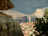
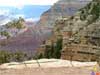
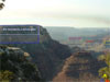
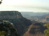
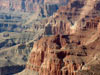
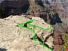
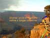
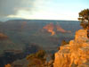
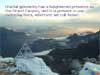
I took this picture on Desert View Drive on the temperamental day of November 30, 2002. (Weather changes can affect the interior of the Canyon dramatically. Small changes in the weather can quickly cause big changes in visibility inside the Canyon do you recognize the familiar ring of Chaos Theory?) The Canyon section deals with visible patterns in the Canyon walls and rim. After viewing the presentation, a few thing in this image should jump out and have meaning. Slides 13-15 (Canyon 2, 3 and
4):
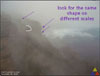
Look for the same shape on different scales. I ve used arrows to point out some shapes that remind me of scallops, also outlined one of them. On slide 14, I outlined a smaller scallop from the edge of the bigger scallop. If we could zoom in, we would probably also notice scallops on the smaller scallop. Slide 15 shows the image with no words. This provides an opportunity to examine the image without animations present. The different masses of land shadow each other. They are all in the same vicinity, probably have about the same rock content, have been exposed to approximately the same weather conditions over a long period of time... Slides 16-17 (Canyon 5 and
6):
I've included this image because the two dogleg sections in the foreground of the Canyon stand out like beacons. They look a lot alike, and there are probably dogleg extensions at their edges. Slides 18-19 (Canyon 7 and
8):
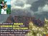
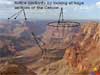
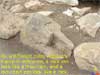
This is the first slide showing the main pattern theme that I have chosen to address in this section. It is a pattern of mutually orthogonal joints that run throughout the Canyon, pointed out to me by a geology professor at ASU. The joints are present on a massive number of scales. The rock is permeated with them, but we only see them after they have been exposed to weathering. They were caused by rock uplift and expansion. It has to do with the way rock releases pressure. The joints begin forming way underground while the rock is uplifting, and expansion continues above ground until all pressure is released. The first release is in the direction of uplift, the second release is mutually orthogonal to the first, and the third and final direction is mutually orthogonal to both the first and second releases of pressure. But pressure is releasing in concert, in an interconnected way, as opposed to: 1) all one direction, 2) all the next direction, and 3) all the final direction. The professor who revealed this to me is introduced in the next slide. For the moment, in this slide, start looking for the pattern highlighted in this image. Slides 20-23 (Canyon 9, 10,
11, and 12):
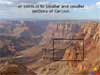
Slide 20 shows Paul Knauth, Professor of Geology at ASU, pictured with his granddaughter. He has been observing this joint pattern for about 30 years. Once you learn to recognize the joints in their different forms, looking at them both in images and in person at the Canyon is very easy. You can see them from anywhere, but they stand out (as a thematic pattern) more clearly from a distance. The joints in the top half of the Canyon are at the same orientation. (All information I am providing is from what Knauth relayed to me, a brief synopsis follows.) In the bottom half of the Canyon: several sets of joints are present at different orientations. Whole sets of joints are superimposed on other whole sets of joints. This has happened because the Canyon bobs up and down like a cork. Lower sections have recompressed and have later been uplifted again, reintroducing the entire expansion process, and sometimes the uplift hasn't been straight up, the rock is uplifted from an angle. From a joints standpoint, the geology from the half-point down is far more complex than the geology from the half-point to the top, so I decided to stick with the top half. Plus, I have never even been to the bottom of the Canyon to see these more complex patterns. Apparently, if you hike to the bottom, you are going to see a different, more complex picture than is shown in any of my images. The mutually orthogonal link provided on this slide goes to a definition and explanation of what it means to be mutually orthogonal. The Grand Canyon link goes to the home page for Grand Canyon National Park. Slides 24-27 (Canyon 13, 14,
15, and 16):
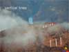
You don't have to look only for blocks, you can look for lines. There are horizontal lines in the form of ridges or cracks, vertical lines in the form of ridges or cracks, and blunt faces. Blunt faces are outermost sections of Canyon, behind or underneath which are many cracks. Imagine looking at a loaf of bread head on. While you can only see the heel, you know there are a lot of slices behind it. This is how it is with blunt faces in the Canyon. Slides 28-30 (Canyon 28, 29,
and 30):
This image was taken on Grandview Trail on Desert View Drive, December 1, 2002. I ve used it because it shows so many right angles and lines, blocks and faces. On the left top-third you can see the edge of a wide, weathered, horizontal crack. Slides 31-33 (Canyon 20, 21,
and 22):
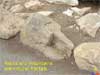
A typical wide, vertical crack is seen here at the rim. Notice the soft edges of the horizontal ridges that run throughout the image along the rim. Slide 32 (Canyon 21) shows a place Knauth pointed out where this section will almost surely break away. We have already noticed that the walls of the Canyon tend toward bluntness. The piece of rock immediately below this section has already released, and the topmost section will someday follow. It will be a terrible thing if someone happens to be standing on it when it falls. Slide 33 shows the image with no words or animation. Notice the shadowing in the rear of the image, and the common ridges shared throughout this area of the Canyon. We are looking at sections of Canyon in the same vicinity that probably have a highly similar rock concentration that have been exposed to similar weather conditions over a long period of time. Is it any wonder that the Canyon looks the same in localized regions?
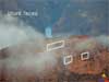
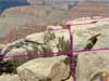
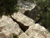
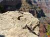
This image begins a Canyon Rim focus on the joints, to make a connection between the rim and walls of the Canyon. I find it to be an amazing image because the blocks in the foreground have such a regular appearance. It was taken in the Mather Point area. It looks to me like someone actually carved the blocks, but it is nature s own carvings that we see here. The rim will recede with time, as more and more joints are weathered and fall, new joints are revealed and weathered, and more blocks fall from the Rim into the Canyon. Slides 35-36 (Canyon 24 and
25):
This image, like the previous image, is from Mather Point. I have outlined some exposed, weathered cracks on the rim. They continue further along in hairline cracks that are at the surface but are not yet weathered. I am highlighting barely enough to bring a few patterns out visually. There is a great deal more to glean from these images than the little bit I highlight. For instance, look at the section leading out into the Canyon in the center of the image: the lines, the blocks, the weathering. We can look at the images and see where blocks are, but often times, we can also see where blocks were and are no longer. Broken extensions of Canyon used to be sections of solid rock with Canyon joints running through them.
This is another instance of what is shown in the previous few images. At this point, try to bring to mind the previous slides. Look at the horizontal and vertical cracks and ridges. Look at the bluntness of the Canyon walls overall, and the myriad individual blunt pieces that make them up. Focusing now on the closest Canyon wall in this image, it is a big, blunt face that is made of blunt faces that is made of blunt faces. There is, furthermore, much more detail than we can see, even if we were scaling the wall with our nose to it. At any given point in time, we can only see what has been weathered. The rest is hidden to our eyes. Slides 38-40 (Canyon 27, 28,
and 29):
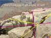
This image is from Desert View Drive. It shows a weathered section of rim with lots of joints. The cracks highlighted in yellow, while orthogonal to each other, are off-orientation to the other localized cracks. Everywhere you look, there are exceptions of one kind or another to prominent patterns. But now look at the lines in the background sections of Canyon. There are four big background sections, and the joint pattern stands out clearly in all of them. Slides 41-42 (Canyon 30 and
31):
Here is another rim example, this one is from the beginning of Desert View Drive en route from the South Rim, a long way yet from the East Rim. Slides 43-45 (Canyon 32, 33,
and 34):
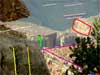
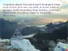
Even after Knauth told me about the joints, I got lost in big views of the Canyon, there is so much information to take in, so many ways to look at the Canyon and experience it. Originally, this image was meant to point out the falling block highlighted in Slide 45 (Canyon 34). I had accidentally placed a line around the text box, but left it there, because the line bordering the box appealed to me. It looked so "right." It took a long time to realize that the rectangular outline on the box looked good because the image is itself filled with rectangular shapes. I later added a slide [Slide 44 (Canyon 33)] to highlight some of the rectangular shapes in the image. Forget about the joints for a moment, just enjoy the rectangles, or whatever it is you see. Perhaps instead of rectangles, you noticed the pyramid-like shapes below the rectangles, pyramidal shapes, by the way, that are made of smaller pyramidal shapes made of yet smaller pyramidal shapes. How many repeating patterns can you find? On Slide 45 (Canyon 34), the arrow is pointed toward a block that is poised at an angle and will someday fall. Slides 46-47 (Canyon 35 and
36):
I have turned the focus to falling blocks. The block in this image has started its way down the Canyon. Winter 2005 has brought a lot of rain and snow to the high country in Arizona that will help blocks like this weather and slip. Slides 48-49 (Canyon 37 and
38):
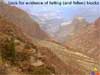
The joint pattern isn't as obvious in this image, camouflaged by lots of things going on in the rock. One particular spot in the image is reminiscent of the previous image, but without a tell-tale block, a clear space left by a fallen block that is no longer around.
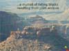
This shows a heavily weathered section with a lot of fallen blocks. Look at the section in the far background, too, where only a piece of the (now) topmost section remains. Some areas of Canyon stay together better than others. I wonder, is it because localized areas have seen harsher weather over time, or the rock in this area is more susceptible to weathering? Whatever the reasons are, this section of Canyon looks like it is falling away faster than some neighbouring sections. As blocks fall, joints at their surface weather. Big blocks weather into smaller blocks, and by the time they arrive in the lower part of the Canyon, many are tiny rectilinear rocks. I asked Knauth: if these blocks are all falling down into the Canyon, won't the Canyon eventually fill up with blocks? He said many arrive at the bottom in little pieces and are carried away by the river, that the river acts as a big conveyor belt that transports the remains of fallen blocks out of the Canyon.
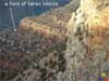
I have called this image field of fallen blocks because of all the blocks that have built up on that single ridge, as if the plateau is holding on to them and won t let them follow their 'bigger' path. Also notice how flat yet knarled the closest section of Canyon wall is. In an up-close view, the joint pattern would hardly be visible, if at all, present as it is in concert with so many other processes. Slides 52-53 (Canyon 41 and
42):
Several areas are highlighted here that show similarity. Notice the ovals that highlight a section of Canyon boundary. Look at the Canyon boundary inside the little oval and then look at the boundary inside the big oval. The smaller section of boundary looks very much like a miniature version of the larger section. If we took a smaller section within the small oval, the same thing would happen.
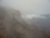
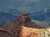
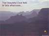
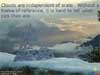
The images used thus far in this presentation have had a frame of reference present, like the skyline, or trees, something that has revealed the relative size of the landmasses in the images. This image has no external frame of reference. It is difficult to determine the size of what we are seeing. We could isolate a smaller section of the image and pass it off as a more massive section of Canyon or a smaller piece than it actually is. This is an example of scale-independence, or scale-invariance. Scale-invariance is crucial to being fractal, no matter the type of fractal structure. I m isolating on natural and geometric fractals in this presentation, but there are a lot of types. Scale-invariance is an inherent property of all types of fractals.
Taken the same day as the previous image, at the East Rim, this image is here because I like it, and it seemed like a nice ending place for the Canyon section. The next sections are shorter. The joints demanded a lot of attention, first of all, to look at them in different ways (looking for blocks versus looking for lines, far away views versus underfoot views on the Canyon rim), and secondly, to consider effects from joints (like falling blocks). This was put together for presentation at Grand Canyon National Park. The Interpretive Education Division of the GCNPS expected that every image and all content should focus on Grand Canyon, so it made sense to have the biggest section be on the Canyon itself. Paul Knauth made the Canyon section worth looking at by telling me about the joint pattern, and taking time out of his busy schedule to answer many questions. Slides 56-58 (Clouds 1, 2,
and 3):
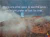
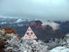
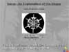
Clouds. How big is a given cloud? You can t know unless there is some external frame of reference in the scene. If you break a cloud into smaller and smaller pieces, at some point you will have something that isn't a cloud. I'm not sure at what point that occurs, but self-similar detail doesn't go on forever in nature. It has a lower limit. What is the upper limit of a cloud, i.e., is there a limit to how big a cloud can get? Limits are assumed to exist with nature, however, a reasonable question to ask might be: how big could the biggest cloud possibly be? Is there such a thing as the biggest possible cloud? There are some huge versions in space made of dust and interstellar gas. A vapour cloud on earth would probably be limited in size by the boundary of our atmosphere. But I don't know, am making no claims about it, am rather throwing this out as a question. Slide 57 (Clouds 2) briefly addresses the appearance of the Sierpinski tetrahedron and provides three links: the first is to my Sierpinski tetrahedron page; the second is to an explanation about geometric fractals on the Arcytech website; the third is to a section on L-systems on the Archytech website, it is a really great site to learn about fractals (the applets are written in Java, and Windows no longer comes with the ability to run it; either the images will come up, or if they don't, a link is on the image to download necessary software). An important thing is to realize that we are not looking for triangles and tetrahedrons in nature. Nature has its own, very different shapes that repeat on different scales and are scale independent. The tetrahedron is in the image 1) because it looks beautiful there, and 2) to highlight and draw attention to the mathematical structure of nature. Slides 59-60 (Clouds 4 and
5):
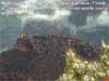
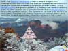
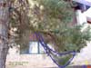
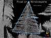
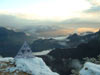
Almost everything in the image is fractal: the snow, the boundary the snow makes on the rock ledge, the ledge (made as it is, of rock), the clouds, the Canyon, the stage-4 Sierpinski tetrahedron, the branches of the tree. The needles on the tree aren't fractal.
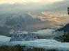
This image is a great complement to some artificial landscape slides created by Richard F. Voss, called making clouds out of mountains. I have a copy of the slides to use for in-person presentations, but cannot use them in the web version. His artificial slides look like a re-creation of a section of this real-world image. Voss created an artificial mountain/canyon landscape, and by changing the lighting, made it into clouds, from the same file, the same Iterated Function System. I haven t said much about clouds, but the point is to look at them and realize that if a piece of a cloud breaks away, it becomes a whole cloud in its own right. The parts are similar to the whole.
This is the second largest section of the presentation. It might better be called Branching , except that it focuses on the branching in trees. It is a large section because I wanted to consider trees with bare branches, and also trees with leaves on them. It can be difficult to see the fractal structure of tree branches when they are covered by leaves. To add to the confusion, leaves are typically not fractal. You have to separate them in your mind from the fractal structure of the tree while looking at the tree, and this can be hard when almost all you see is leaves. They do have fractal properties, however. The veins that run through them are fractal, and there are times when their edges have a fractal boundary, but leaves are generally not made up of little leaves that look just like them. Slides 63-65 (Trees 2, 3, and
4):
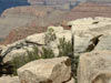
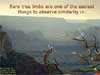
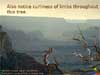
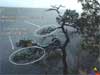
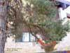
This is the easy way to look at trees, is when they have bare branches. I believe one of the Interpretative Rangers said this tree is a Juniper, seen frequently in the Canyon. From tree to tree, there are different characteristics between the limbs, such as the shapes of the intersections, from wide U shapes to sharp V's and everything in-between. Pretty much, whatever the shape at an intersection in a given tree, that shape will hold in the intersections throughout the entire tree. The tree in this image also has curly branches. Notice that there isn't just an isolated branch or two with a curly limb, this is a characteristic pattern of the limbs throughout the tree.
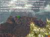
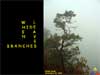
This image covers a lot of ground, across several slides. This is the only image for which I will break apart the slide notes. As of 03/20/05, the notes and presentation have barely been put up. The notes for this image in particular need a lot of work. They may be a struggle to read. In both the tree and the (Sierpinski) tetrahedron there is fractal structure: scale invariance, small parts that look like big parts, and exponential growth an overall fractal pattern. In spite of commonalities, there are differences between the way these two objects grow that are representative of differences between geometric fractals and natural fractals generally. Some differences include that the Sierpinski tetrahedron uses an exact shape (a regular tetrahedron), the growth pattern between stages is exact, and the growth can feasibly go on forever. Contrast this with the tree, where both the similarity between the shape of the limbs and the growth pattern between stages is approximate rather than exact, plus, the tree has a limited number of stages of growth. It "tips out". The tree shows approximate, or statistical self-similarity. Geometric fractals, on the other hand, show exact self-similarity. One qualification: self-similarity only really happens in the limit, i.e., at infinity. Somewhere, at infinity, the Sierpinski tetrahedron will achieve self-similarity, where every little part will be identical to the whole structure. It is a kind of "out-there" thought!
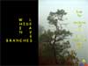
This step begins the process of following a connected path through 4 stages of growth of a Sierpinski tetrahedron. There is a single opening highlighted in this slide, the one and only biggest opening. At any given stage of growth, there is a single biggest opening. Notice there are a few choices for the second biggest opening, 4 to be exact. Whatever path is chosen, much detail and growth of the structure will be left behind along the way, and the numbers will exponentially explode as growth progresses. The link on this slide is to the Sierpinski tetrahedron lab page on the Yale Fractal Geometry website. It is a good lab for older grades, say 6th and up. It addresses more than building, it lends perspective to what is happening. It might also be the case that Yale's building method (using envelopes to make the tetrahedrons) would work great for grades as low as 2nd or 3rd, I just don't know.
There were 4 same-size choices for the second largest opening, all were on a connected path, I chose one, leaving 3 openings behind. There are 4x4=16 next largest openings, where only four are touching a connected path. One will be chosen, leaving 15 same-size openings behind. Next will be 4x4x4=64 smallest openings, again with four touching our path. One opening will be chosen and 63 same-size openings left behind.
Following what appears to be a small path only 4 stages of growth so far we have already left behind 3+15+63=81 openings total. Beyond this image, the next stage the stage-5 has 128 openings to choose from, with (as always with Sierpinski's tetrahedron) 4 openings touching a connected path. Sierpinski's tetrahedron grows in an identical form from stage to stage. The shape is a regular tetrahedron, and it always grows in powers of 4. Each stage is 4 of the previous stage set tip-to-tip. The edge-length either doubles at each stage, or the lengths of the individual tetrahedra are halved at each stage, depending on the growth method chosen. The link on this slide is to the Yale Fractal Geometry website's Self-Similarity page.
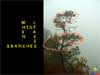
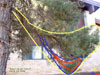
Now we've switched from the tetrahedron to the tree. We're following a connected path through the tree. Five massive branches lead off the trunk at the first intersection (one branch is hidden from view by the front most branch). Each intersection along the path is marked by a yellow oval, called a node. The possible paths leading off the node are highlighted, where only one limb is followed to the next node. With the first path choice, 4/5 s of the tree is left behind. The next intersection has 4 branches leading off it, one path is taken, leaving (4/5)x(3/4) of tree behind. At the 3rd intersection, there are only three limbs. One limb is chosen, the other two abandoned, leaving (4/5)x(3/4)x(2/3) s behind. Next intersection, there are only 2 limbs, leaving a total so far of (4/5)x(3/4)x(2/3)x(1/2)=~80% of the detail of the tree behind. When stages 5 ane 6 are included, plus two additional stages that were too small to highlight on the slide, each with two branches to choose from in this way-oversimplified example, approximately 99% of the tree is left behind. The slide includes a link to one of Yale's pages about natural fractals and approximate self-similarity.
Notice that the tree isn't growing in exactly the same way from stage to stage. Although the number of limbs is growing exponentially, the rate of growth between stages is decreasing, growth is surging forward with limits, probably because nature is efficient. The limbs have to fit into a real-world space that includes constraints of size and proportion. Leaves have to fit on its many branches. If 4 or 5 limbs had branched off at every single intersection along the way, there wouldn't be room for all the limbs much less any leaves! Assuming that similar growth is taking place throughout the tree, at stage 8 this tree will have 5x4x3x2x2x2x2x2 limbs, or approximately 2,000 limbs (found by multiplying the number of limbs at each stage along the path, and including the two stages at the top that were too small to highlight). I can't tell, there may be an intersection of branches hidden behind the tetrahedron, a 3-branch node. If this is correct and the number of intersections is really 9, then the number of limbs increases to somewhere around 5,000-6,000 in the real tree in this image. Suppose the tree had grown at a consistent rate exponentially, like the tetrahedron. At the first node there were 5 branches. If it had continued at a rate of 5 branches per intersection, the number of limbs at stage 8 would be 5^8 = 5x5x5x5x5x5x5 = 390,625 limbs! And if there are really 9 stages to this tree, 5^9 = 5x5x5x5x5x5x5x5x5 would be 1,953,125 limbs! It simply couldn't be. So real trees in nature show exponential growth, yes, but it shows up in a different way than in the Sierpinski tetrahedron, and geometric fractals in general. This doesn't invalidate the fractal structure that they share. A small piece of a tree closely resembles a bigger piece of the same tree. Both Sierpinski s tetrahedron and the tree look very much like the parts that make them up, even though they reveal different patterns of fractal growth. It should be noted that some biological systems, bacteria growth is one example, model classic exponential growth, but when that happens, to whatever degree it happens, it is because the natural system can handle it. Otherwise, nature would make adjustments, similar to the tree in this example.
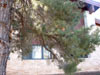
Try to see the content of the previous slides without any animations. Or maybe just enjoy the image without thinking about anything. I m trying to make mathematical connections in nature not to take away the aesthetic experience of nature, rather to blend the two. Slides 73-74 (Trees 12 and
13):
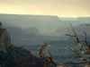
This image points out the similarity in shape between a small and large section of bare branches, and further compares a bare and branched section of limbs. It is one of my favourite images from the Canyon, taken December 1, 2002, on Hermit s Route. Slides 75-77 (Trees 14, 15,
and 16):
"When leaves hide branches." When tree branches have leaf coverage, it can be difficult to examine the shapes of the branches. You have to look for little sections of tree that resemble each other, and sections within sections that resemble each other. You also need to satisfy yourself that this is true not because of the leaves but because of the branches underneath them that the leaves are growing on. This was a sticking point for me. For at least two years after learning about fractals, I had terrible difficulties with leafed trees. It is due to this long personal difficulty that I am including this section. If it was a stumbling block for me, it might be a stumbling block for other people, too. Slides 78-80 (Trees 17, 18,
and 19):
The words in parenthesis on this slide are from Root Gorelick, a faculty research associate with the School of Life Sciences at Arizona State University. There was nothing about terminal organs in this presentation until he pointed out the connection. These slides show a tree with brushy features where the branches underneath are almost not visible. The slides for this image 1) reinforce the message of the slides from the previous two images, and 2) focus on leaves not typically being fractal. They are at the tips of the tree. Leaves are terminal organs and as such do not reproduce little copies of themselves. On the other hand, the vein structure in leaves reveal fractal branching patterns, and some leaves have fractal boundaries, meaning the the edge might reveal the same shape at smaller and smaller scales of detail. There are so many distinctions to make, or so it seems to me. The point here is that leaves are generally not made up of little leaves that look just like them. The fern, however, is a big, leafy plant with leaves that are made of leaves that are made of leaves that have the same shape. This holds with the asparagus fern too, although the pattern is much harder to see. You could think of an asparagus fern as a plant made of winding wide-bristled brushes made of smaller winding, wide-bristled brushes made of smaller winding wide-bristled brushes. The brushes and bristles circle like a helix around whatever stem they are coming off of. The fern family, though, is an exception. I've included links to images of them since they are not part of the Canyon decor (that I have seen) and are therefore not seen in the presentation, I bring them up only in these notes. Leaves are generally not reproductive. It may be the case that ferns are not technically "leaves." Slides 81-85 (Trees 20, 21,
22, 23, and 24):
Nothing new is introduced in this slide. It serves to support the previous slides. The image was taken in the school yard of the Grand Canyon on-site school. To me, these branches resemble a boot, and I ve followed the boot shape through some smaller sections of branches. The huge branch is made up of little branches that have a similar appearance, that when put together, form a bigger shape that resembles the smaller shapes. The branches are pretty much hidden by leaves that clothe them. People wear clothes every day. We don't have to see people without their clothes on in order to recognize them, and we don't have to see trees without leaves on them to recognize the fractal branching of the limbs underneath! Slides 86-90 (Trees 25, 26,
27, 28, and 29):
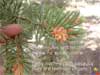
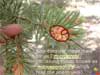
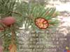
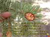
This set of slides is important. It follows the theme of leaves being terminal organs and not fractal. The really important part of this group of slides is that the image shows a fractal structure in a male cone containing bracts with only one level of substructure. The male cone reproduces copies of itself on one scale in the form of bracts that the terminal organs (the needles on the tree) grow out of. It is frequently said that nature shows a limited number of similar scales. Here is the bottom rung, the least you can have, one stage of similarity. The pattern of mutually orthogonal joints running throughout Grand Canyon, on the other hand, is present on a magnificent, uncountable number of scales (it is finite, but it is a huge number). We have natural systems like clouds and the Canyon with a magnificent number of scales, systems like trees and bushes with a nice handful of scales, and here are these male cones with only a single scale of similar substructure. (I should point out that some people might take issue with whether or not one stage of similarity in this male cone is enough to say it is fractal. There will probably be dissenting views.) Slides 91-94 (Lightning 1,
2, 3, and 4):
I ve included lightning because it s enigmatic to look at and exciting to children. In my in-person (i.e., not a web version) presentation, I have an image of lightning striking the North Rim of Grand Canyon taken by professional photographer Mike McFadden. Slide 91 (Lightning 1) links to the image on McFadden s web page. The structure of lightning is self-similar. As you zoom into it, what you see is more lightning. As an aside, lightning strikes produce beautiful branching patterns. Peter Ledlie took the picture shown on these slides. Ledlie s url at the bottom of Slide 91 (Lightning 1) shows pictures of him using equipment to produce lightning strikes in his laboratory.
This is one of my favourite images, and it is only seen in this one slide. I like the way the Rim boundary stretches into the distance. Fractal boundaries is a terrific topic for Grand Canyon. It is the topic that the Rangers seemed to identify with the most, especially relating to hiking and maps in the bottom of the Canyon. I hope to include some of their perspectives and experiences as they apply to fractal geometry. I haven t even been to the bottom of the Canyon, have only seen it from the top, aside from a couple of very short walks in. This section shows the greatest potential for expansion. Slides 96-99 (Boundaries 2,
3, and 4):
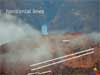
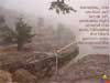
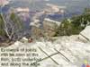
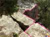
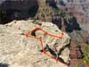
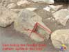
An extended fractal boundary has been created along the Canyon rim by a block that is getting ready to fall. The block has separated and tilted forward, and I have followed the big crack it has made with an imaginary measuring stick. In Slide 97 (Boundaries 3), the measuring stick is halved, and more detail is captured. In Slide 98 (Boundaries 4), the measuring stick is halved again, and now we are beginning to closely follow the path of this separation. If the measuring stick were shortened again, and again, we would continue to follow the path more closely. As a rough path is increasingly "hugged", the distance around it gets longer, as more detail is captured. The rim boundary of Grand Canyon is constantly changing. On another note, look at the saw-tooth edge of the dark section of Canyon in the background. The pattern is tiered: in smaller scale above, in larger scale below.
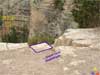
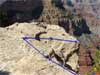
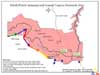
I applied a measuring stick to a Hawkwatch International map of Grand Canyon, with Hawkwatch s permission. Slides 101-103 (Boundaries
6, 7, and 8):
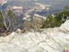
A section of rim boundary is outlined and a measuring stick applied to it. Look at the numbers on Slide 101 (Boundaries 6) that compare the measuring stick to coastline length. They tell a compelling story. The length of the Coast of Britain is a problem that really occurred, recounted in the link provided. Slides 104-107 (Boundaries
9, 10, 11, and 12):
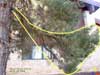
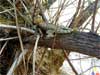
Tree trunks are fractal boundaries, where the fractal dimension is dependent upon the roughness of the trunk. A rougher trunk has a higher fractal dimension. This looks like a trunk with considerable roughness. The pattern of the trunk itself, the shape of the pieces that make it up, also shows statistical self-similarity, in that small sections of bark resemble larger sections of bark. The link on the slide goes to a website at the University of Manitoba called Fractals in the Biological Sciences. Tree trunks are mentioned in their section 1.3. The link, however, goes to section 5 where habitats are discussed. There is a lot of space for tiny bugs on this trunk that bigger bugs can t even get to. Tree trunks play an important role in supporting biological diversity. I recommend reading two of their sections entirely: sections 1 and 5, just skim through the many fractal applications in biology that are briefly described. Slides 108-109 (Boundaries
13 and 14):
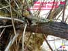
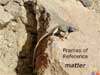
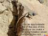
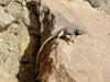
This trunk is much smoother than the last one and will have smaller fractal dimension. It will still be a longer distance around it for a bug with shorter legs. Slides 110-112 (Frame of
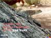
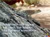
Reference 1, 2, and 3):
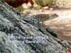
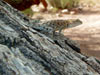
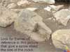
A quarter or a dollar bill on this rock would give a concrete idea about the quantity of rock in the image, because it would be an exact, external frame of reference. We have to guess about the size of the lizard, but at the same time, we know it isn't a Godzilla. At least the lizard gives us a general idea about how much rock we are seeing in the image. Slides 113-116 (Frame of
Ref. 4, Rocks/Mountains 1, 2, and 3):
This is a plain little image that has been very useful. Slides 117-118 (Snow 1
and 2):
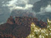
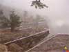
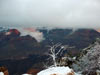
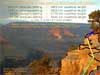
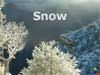
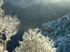
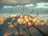
This picture was taken on New Year s Day 2005 at around 9:00 a.m. in the Mather Point area. It had snowed overnight. I couldn't find any links that talk about the fractal properties of accumulated snow, but there are a lot of links that talk about snowflakes. Going backward to trees for a moment, look at the wide forks formed by the branches in the tree on the left, and how the pattern follows all the way through the tree. It looks as though the limbs are reaching way out to the side and up.
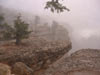
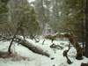
This is a favourite snowy image taken on Desert View Drive on November 29, 2002. Slides 120-122 (Snow 4,
5, and 6):
This section is verbatim from the Yale Fractal Geometry pages, with a link provided to the page it came from. If you click on snow at the bottom of the page, it takes you to a group of links for a few more of their pages on snow. It is a big site to maneuver, but they are very good about keeping individual pages within the site small. I keep linking to pages on the Yale site in order to introduce and reintroduce people to it, because the information provided is trustworthy. It is such a massive site, if you want to seek something out on the Yale Fractal Geometry web pages, my advice is to go to Google (www.google.com), and in the search box, type the desired term and then add: + Yale + fractals. This way, Google will bring up results on their website first. It s what I do most of the time.
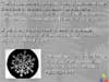
This is one of Wilson Bentley s images. The fractal structure is triangles made of triangles. Slides 124-126 (Conclusion
1, 2, and 3):
Hopefully at this point, an overall sense has been developed about fractals in nature. If you have looked at the entire presentation and have visited the links provided, perhaps a precursory, comparative understanding has formed with regard to geometric fractals as well. It s a huge topic. My wish for viewers is that the journey be enjoyable while perspective is acquired.
In order of sequence of events: Summer 2003 Heinz-Otto Peiten and Richard F. Voss, mathematics professors at Florida Atlantic University (Peitgen is also with the University of Bremen) held a two-week NSF Technology in the Classroom summer institute on working with PowerPoint, which I attended. Spring 2003 through November 2004 knowing ahead of time that I would learn to use PowerPoint at the above-referenced NSF institute over the summer, I began thinking about introducing a presentation about natural fractals into a national park, to make a case for bringing math education about fractals into what I think is a very appropriate environment for it, from multiple angles. Not until Winter 2004 did I approach the Grand Canyon National Park Service about it. Their response was non-committal yet open-ended. Preparatory conversations with the Division of Interpretative and Resource Education ensued, and it was decided that I would give a trial run presentation at their on-site school. Spring 2004 Marilyn Carlson, mathematics professor and Director of CRESMET at ASU, provided the loan of a laptop. Spring 2004 Richard Voss loaned me the use of his making clouds of of mountains images for in-person presentations. His images aren't in the web version, but they were an important contribution to the project overall and helped it go forward, making connections between artificial and real-world fractals in such a beautiful way. Whatever is on the internet is unfortunately out there for the taking and there would be no way to keep his images safe. May 2004 I gave the trial run fractals in nature presentation at the Grand Canyon on-site school. It was very different from this one. At that time I didn't even know about the joints. The decision was made to go forward on something totally canyon-focused. Summer 2004 Paul Knauth, geology professor at ASU, told me about the Canyon joints in a series of meetings, after which I began putting the presentation together. He took time out of his schedule more than once when he was wildly busy with grant writing and other pressing projects. Fall 2004 Don Jones, mathematics professor and Chair of Undergraduate Studies with the Department of Mathematics and Statistics at ASU, went through the initial draft and offered several content-related suggestions, all of which were incorporated. October 2004 Charles Wahler, Acting Assistant Chief of Interpretative and Resource Education with the GCNPS, offered suggestions, all incorporated. November 2004 I gave a trial run presentation at the Mathematics and Cognition Seminar, where it was critiqued by professors from mathematics, psychology, biology, human and family studies, and philosophy. Many good suggestions were offered, and considerable changes ensued. One example in particular: the insight offered about terminal organs on slides 80 and 86-90 came from Root Gorelick, a faculty research associate with the School of Life Sciences. December 2004 The presentation was given as a special program at Grand Canyon National Park on New Years Eve 2004 and New Year's Day 2005. Several interpretive rangers had interesting comments related to their experiences with the Canyon which I plan to follow up on and incorporate at a later time. February-March 2005 Considerations for placing this on the web were size of download, providing slide notes, and generally trying to put it up in such a way that people unfamiliar with the subject matter could navigate it alone and choose to project it in a classroom if so desired. March 2005 Reimund Albers from the University of Bremen offered suggestions for the web version related to animations on some slides and incorporating higher quality images. It was around 7MB's at that time, and Reimund found that it didn't project well, so I replaced 480x640 medium quality images with 600x800 high quality images, increasing the file size to 15MB's. Striking a balance between file download size and viewing quality has been a struggle. Photography student and co-worker Brian Radspinner has helped all along, but even more than usual with the web version, answering questions about images and html code. March 2005 Paul Bourke, Visualization Research Fellow with the Swinburne Centre for Astrophysics and Supercomputing, looked it over and most of his suggestions focused on my animations and the appearance of the text. All of his suggestions were incorporated, after which both of us made the presentation available from our websites: in PowerPoint, and a Keynote version for people with Macs. It is being readied for pdf right now. If the presentation were accessible only from my website, it would stay relatively obscure for a long time. By putting it on Paul's site, too, it it went straight to the top of some big search terms in Google. Plus, it is accessible from Paul's fractals page which comes up at or near the top of a great many searches. The difference is like being in a row boat in a lake with no breeze versus white-water rafting on the Zambesi. by mid-April 2005 it should be up in pdf form. Renate Mittelmann, Computer Research Specialist with Mathematics and Statistics at ASU said anyone should be able to view a pdf version. Different versions have different benefits. There are some sacrifices with pdf, but people running Linux will at least be able to view it in this form, and others may even prefer it. Renate and Jialong He, Information Technology Specialist, always find time to answer questions even while everyone is bombarding them with requests. If you the viewer find that something doesn't make sense, please feel free to offer suggestions. If changes need to be made, I need to know about it and make them. If your suggestion generates a content-based or appearance-based change, your name will be added to this list along with everyone else's. Feel free to email me with comments: gayla.chandler(at)asu.edu. The subject line should read "Grand Canyon presentation". |