Box counting fractal dimension of volumetric dataWritten by Paul BourkeApril-May 2014 Introduction
The box counting, or more precisely "cube counting" estimate for fractal dimension (FD) is also known as the Minkowski-Bouligand dimension or Kolmogorov dimension. The basic idea arises by considering the length, area, and volume of Euclidean objects such as a line, plane, and cube. In one dimension consider a curve and a ruler of length s. If one counts the number of rulers N(s) required to cover the curve as s decreases then the relationship will be N(s) proportional to 1/s1. Similarly in 2 dimensions if we count the number of squares of side length s required to cover a surface then the relationship will be N(s) proportional to 1/s2. And finally in 3 dimensions using a cube of side length s and counting how many such cubes are required to fill a volume the relationship will be N(s) proportional to 1/s3. This is equivalent to our understanding of length, area, and volume. If we double the size of a one dimensional object the length increases by a factor of 21, if we double the size of a 2 dimensional object the area increases by a factor of 4 (22), and if we double the size of a 3 dimensional object the volume increases by a factor of 8 (23). The superscripts in the above correspond to the notion of dimensions 1, 2 and 3 respectively. The above relationship can be generalised for fractal (fractional dimensional) objects by using the relationship N(s) proportional to 1/sD. If N(s) is computed across a range of s then there should be a linear relationship between log(N(s)) and log(1/s), the slope being the estimate of the fractal dimension. Absence of a linear relationship implies the object isn't fractal or it could be a multifractal. Algorithm
Estimating the box counting FD of a 3D object involves counting the number of cubes N(s) of side length s required to cover the object. The FD is the slope of log(N(s)) vs log(1/s). One of the challenges is to decide how the data will be prepared and presented to the software. While image formats are well established to represent data for 2D FD estimates, the standards for volume data are less standardised. The choice used here is a simple raw format with a minimal header that contains the dimensions of the volume. The format chosen is the same used by the Drishti volume rendering software. This is a convenient because it is supported by the powerful Drishti data import software, allows simple checks to be performed on the volumes being analysed, and is quite easy to create using software one might write oneself. The following is a simplistic code snippet showing how the volume may be exported to the raw volume format chosen. In particular it defines the ordering of the x,y,z axes. The first byte defines the data type, 0 referring to an unsigned char. At the time of writing other datatypes are not supported. The volume dimensions are stored as integers (4 bytes). As such the header is 13 bytes followed by the raw volumetric data, namely nx*ny*nz bytes.
   // The volume has dimensions nx,ny,nz
   // The volume is of type unsigned char, for example, unsigned char ***vol
   fputc(0,fraw);
   fwrite(&nz,sizeof(int),1,fraw);
   fwrite(&ny,sizeof(int),1,fraw);
   fwrite(&nx,sizeof(int),1,fraw);
   for (k=0;k<nz;k++) {
      for (j=0;j<ny;j++) {
         for (i=0;i<nx;i++) {
            fputc(vol[i][j][k],fraw);
         }
      }
   }
The algorithm is quite straightforward: over a range of offsets (see later) and over a range of cube sizes s, compute the number of cubes which contain a voxel within the object under study. One immediately realises that there needs to be a definition of what voxel values constitute the object, this is also known as thresholding and sometimes as segmentation. The key point is that box counting does not apply to a volume with continuous values but rather only to a binary volume. This thresholding can be performed external to this box counting software or by using the -level or -range command line options, see software usage below. The algorithm may be written in pseudo-code as follows:
   for all offsets
      for all box sizes s
         N(s) = 0
         for all box positions
            for all voxels inside the current box
               if the voxel is part of the object
                  N(s) = N(s) + 1
                  stop searching voxels in the current box
               end
            end
         end
      end
   end
Case study 1: Menger sponge
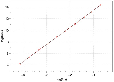
Before applying any fractal dimension estimator to data of unknown FD it is important to test the algorithm against fractals of known dimension. In the case of the 3D Menger sponge illustrated below the FD is given by log(20) / log(3) = 2.7268, this happens to be both the FD of the volume as well as the surface. 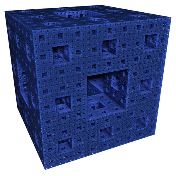 The raw results reported by the software are shown in the table below. The first column is the box size s. The second column is the number of boxes of that size required to cover the object N(s). The third and fourth columns are log(1/s) and log(N(s)) respectively, the slope of these is the estimate of the box counting FD. s N(s) log(1/s) log(N(s)) ---- ---------- ---------- ----------- 2 14348848 -0.69314 16.4792 3 3200000 -1.09861 14.9787 4 2432160 -1.38629 14.7043 6 723680 -1.79176 13.4921 9 160000 -2.19722 11.9829 13 104736 -2.56495 11.5592 19 37044 -2.94444 10.5199 28 13635 -3.33220 9.5204 42 4400 -3.73767 8.3893 63 1458 -4.14313 7.2848 94 432 -4.54329 6.0684 141 200 -4.94876 5.2983 211 64 -5.35186 4.1588 The graph of the raw data above is shown below and the measured slope is 2.62. For these known cases one doesn't expect a perfect match to theoretical because the image is only an approximation to the real fractal form. 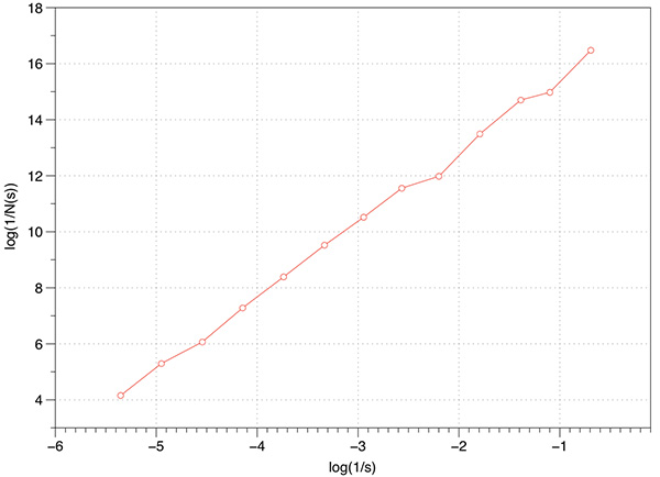
In the above estimation a maximum of 1000 offsets were used to find the minimum coverage. Note that for box sizes 3 and 9 there is a round number of N which is due to the Menger sponge being aligned to voxels in it's generation. Just using these two data points the FD estimate would be the expected value. However, as it happens these two points are an artefact of the way the sponge was created, as such they actually serve to bias the result lower than the expected value. Case Study 2: Cantor dust
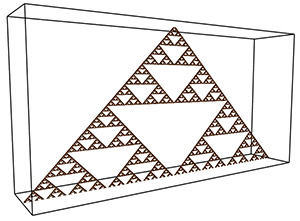
Another 3D fractal of known FD is Cantor dust, this is formed in 1D by starting with a line segment and removing the middle 1/3 segment and iteratively for all subsequent line segments. 
This can readily be extended into 2D and 3D. The FD for the 3D case is log(8) / log(3) = 1.8928. 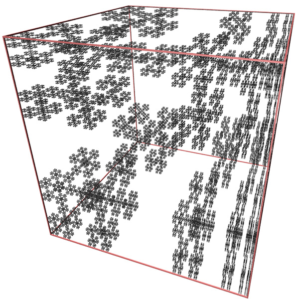
The graph of log(N(s)) vs log(1/s) is shown below, a maximum of 1000 offsets were tested. The measured slope is 1.88 which is extremely good agreement with the expected value. 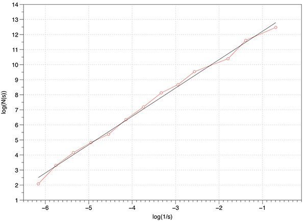
Accurate estimates of the FD require one finds the minimum number of boxes that cover the object. Few algorithms seem to consider this, perhaps because it greatly increases the processing time required. In the implementation here, and since the data is based upon regular volumetric data, the origin for the 3D tile of boxes is randomly offset in the three dimensions. That is, for a particular box size many possible coverings are considered and the minimum is recorded for the subsequent slope estimation. A simple example is shown below in 2 dimensions, the origin for the boxes on the left gives N(s) = 4 whereas the minimum box count required to cover the object is N(s) = 2. 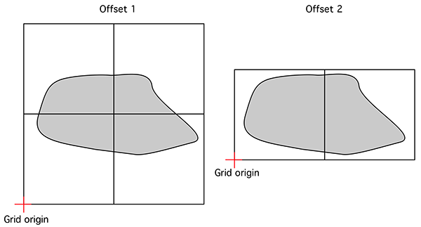
The effect on the FD estimate by using offsets is explored below using the cantor dust example. As the box size increases there is more likelihood that lower box coverings will be found so the effect will be to generally raise the FD estimate. The small box sizes are less likely to change with higher offset counts. Put another way, without considering offsets any estimate of FD will be biased towards lower values. Low number of offsets additionally results in more variation of the slope and thus less reliable slope estimates. An even more rigorous implementation to find the minimal coverage would include considering a range of angular orientations for the coordinate system. This not only adds another three degrees of freedom and the corresponding computation time, but also raises some questions around the fact that sample boxes no longer align in a discrete way with the volumetric data. 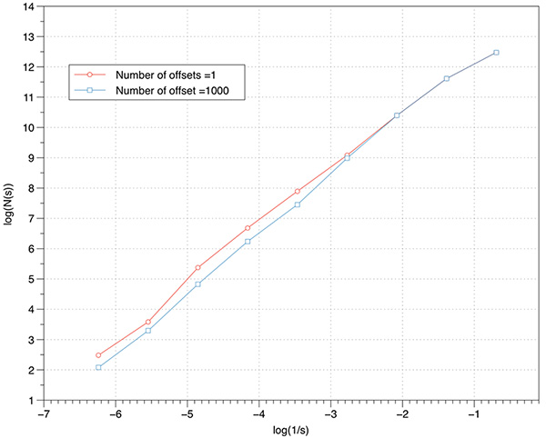 Non-fractal tests
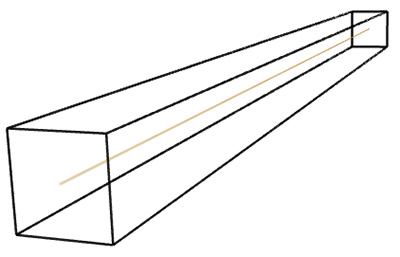
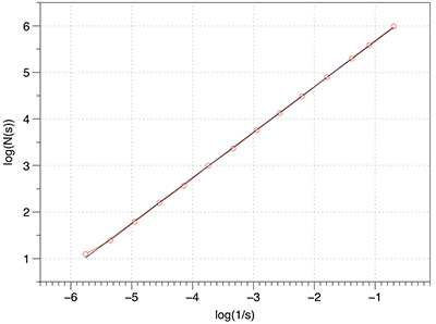
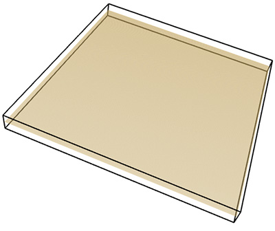
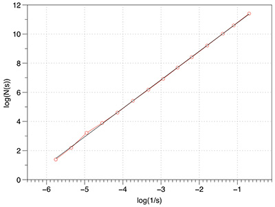
The three tests conducted below were for a line, plane, and a solid box. Of course the dimension of each of these is known, namely 1, 2, and 3 respectively. As shown below the estimates from the software were as close as can be expected for a limited sample (volume) size. Line segment: FD estimate of 0.98.
Plane: FD estimate of 1.96.
Box: FD estimate of 2.95.
Effect of volume resolution
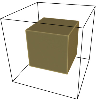
As one might expect, the higher the volume resolution the better the FD estimate will be. The following graphs are for 1000 offsets for a cube object ranging from 20x20x20 to 640x640x640. As expected the variation of the slope reduces as the resolution increases. 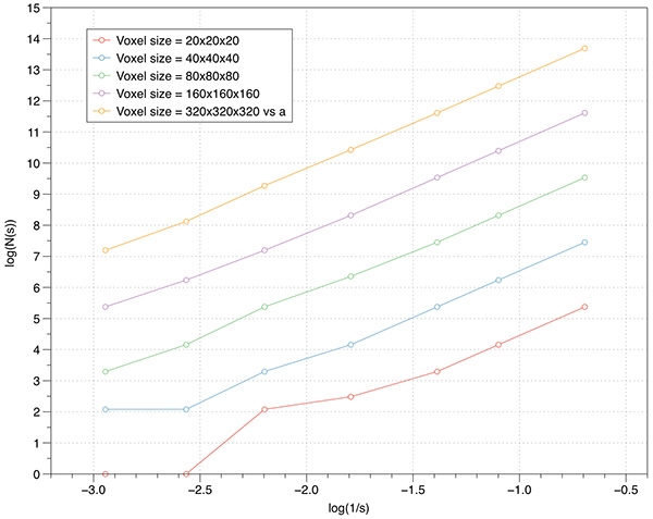 Levels
Most volumetric data is of course not binary, many are continuous functions arising from CT or MRI scans. While volume processing software allows one to segment and otherwise threshold data, some of that is supported within the box counting software itself. One option is to set the level at which a voxel is decreed to be solid or not. By default since volume voxels are single bytes then the values range from 0 to 255, the threshold is taken to be 128. So one may run simple scripts that scan across a range of threshold levels computing the FD for each level. 
An example of this is demonstrated for the volume above. The application of this is to scan the volume for threshold ranges of interest from a FD perspective. 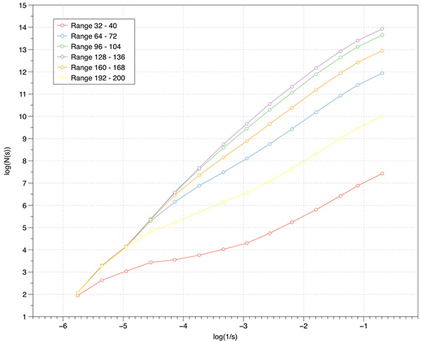 Case study 3
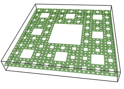
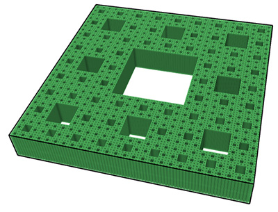
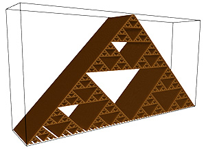
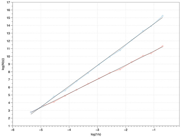
Further tests can be performed using 2D fractals with known FD, for example the Menger carpet. The theoretical FD is log(8) / log(3) = 1.8928. An extruded Menger carpet would have a FD of 1 + log(8) / log(3) = 2.8928. The measured slope from the Menger sponge and extruded Menger sponge is 1.8 and 2.78 respectively.
Case study 4
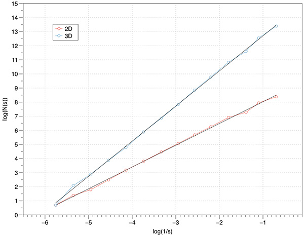
Theoretical FD for the 2D case is log(8) / log(2) = 1.58, measured FD is 1.54. The theoretical FD for the extruded case is 2.58, measured is 2.5.
Usage: volboxcount [options] volfilename
Options:
   -bmin n       minimal box size (default: 2)
   -bmax n       maximum box size (default: largest dimension)
   -bfact n      box size factor (default: 1.5)
   -level n      voxel level above which defines the object (default: 128)
   -range n1 n2  voxel range defining the object (default: 128 255)
   -mset n       Maximum number of offsets used (default: 10)
Notes:
Worked example
In what follows is a complete worked example showing all aspects of the software and analysis. The dataset being used can be downloaded from here: foam.raw. Rendered with Drishti and a transfer function centered on the value of 16 is illustrated below. 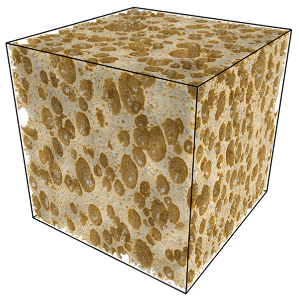 The command line is as follows volboxcount -bmin 4 -bmax 50 -range 10 20 10 -mset 1000 foam.raw The standard output is shown below, note that for a particular box size the multiple box counts occur when a lower number is found during the offset search. Computing box size: 4, Offset: 0 / 64, Minimum box count: 66316 Computing box size: 4, Offset: 1 / 64, Minimum box count: 65948 Computing box size: 4, Offset: 3 / 64, Minimum box count: 65520 Computing box size: 4, Offset: 6 / 64, Minimum box count: 65199 Computing box size: 4, Offset: 17 / 64, Minimum box count: 64923 Computing box size: 4, Offset: 63 / 64, Minimum box count: 64468 Computing box size: 6, Offset: 0 / 216, Minimum box count: 27134 Computing box size: 6, Offset: 1 / 216, Minimum box count: 27010 Computing box size: 6, Offset: 2 / 216, Minimum box count: 25829 Computing box size: 6, Offset: 37 / 216, Minimum box count: 25779 Computing box size: 6, Offset: 74 / 216, Minimum box count: 25678 Computing box size: 6, Offset: 197 / 216, Minimum box count: 25613 Computing box size: 9, Offset: 0 / 729, Minimum box count: 8657 Computing box size: 9, Offset: 4 / 729, Minimum box count: 8589 Computing box size: 9, Offset: 6 / 729, Minimum box count: 8248 Computing box size: 9, Offset: 71 / 729, Minimum box count: 7871 Computing box size: 13, Offset: 0 / 1000, Minimum box count: 3354 Computing box size: 13, Offset: 1 / 1000, Minimum box count: 3349 Computing box size: 13, Offset: 2 / 1000, Minimum box count: 3345 Computing box size: 13, Offset: 3 / 1000, Minimum box count: 3343 Computing box size: 13, Offset: 5 / 1000, Minimum box count: 3132 Computing box size: 13, Offset: 6 / 1000, Minimum box count: 3131 Computing box size: 13, Offset: 8 / 1000, Minimum box count: 3127 Computing box size: 13, Offset: 11 / 1000, Minimum box count: 2924 Computing box size: 13, Offset: 20 / 1000, Minimum box count: 2921 Computing box size: 13, Offset: 33 / 1000, Minimum box count: 2920 Computing box size: 13, Offset: 243 / 1000, Minimum box count: 2735 Computing box size: 13, Offset: 352 / 1000, Minimum box count: 2733 Computing box size: 13, Offset: 623 / 1000, Minimum box count: 2732 Computing box size: 13, Offset: 799 / 1000, Minimum box count: 2731 Computing box size: 19, Offset: 0 / 1000, Minimum box count: 1208 Computing box size: 19, Offset: 2 / 1000, Minimum box count: 1100 Computing box size: 19, Offset: 3 / 1000, Minimum box count: 1098 Computing box size: 19, Offset: 10 / 1000, Minimum box count: 1000 Computing box size: 19, Offset: 14 / 1000, Minimum box count: 999 Computing box size: 19, Offset: 348 / 1000, Minimum box count: 998 Computing box size: 28, Offset: 0 / 1000, Minimum box count: 447 Computing box size: 28, Offset: 2 / 1000, Minimum box count: 392 Computing box size: 28, Offset: 3 / 1000, Minimum box count: 343 Computing box size: 42, Offset: 0 / 1000, Minimum box count: 125 The raw data is as follows: s N(s) log(1/s) log(N(s)) ---- ---------- ---------- ----------- 4 64468 -1.38629 11.0739 6 25613 -1.79176 10.1509 9 7871 -2.19722 8.97094 13 2731 -2.56495 7.91242 19 998 -2.94444 6.90575 28 343 -3.33220 5.83773 42 125 -3.73767 4.82831 Graphed data shown below, FD estimate is 2.7. 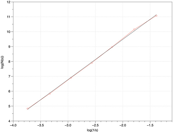 References
|
