Delta codingA simple compression scheme for audio, eeg, and general time series data files.Written by Paul Bourke May 1998
There exist many compression schemes, the right one to use in a particular situation depends largely on the type of data being compressed. The greater the compression ratios the more dependent the method tends to be to characteristics of the data. So for example, greater compression ratios can be achieved if run length encoding is applied to black and white drawings than if it is applied to colour photographs. JPEG gives better compression ratios for photographs than a general compression method such as GZIP. Many compression algorithms achieve very large compression ratios by "changing" the data. The changes are often cleverly made so that they aren't noticeable, for example, JPEG degrades the image in ways that the human visual system is not sensitive to. Some audio compression methods approximate the original signal with considerations of the limitations in the target playback system. A requirement with many recordings for scientific analysis is the data must not be degraded in any way, this is often referred to as a lossless compression method. In many time series derived from sampling continuous signals, the transition between samples is often much less than the total range available for the samples. For example, an acquisition system might store each sample in 16 bits, however since each subsequent sample usually changes slowly the difference between two samples can be stored in fewer bits. This is the essence of delta coding, store the changes instead of the absolute values. Of course the first sample needs to be stored in full resolution and occasionally there might be a larger transition. To cope with this a flag is normally used to indicate whether or not the next sample is a delta or absolute value. One disadvantage of delta coding is that to know the value of the signal at any point in time one has the read (know) all the previous values. ExampleA particular example will be used below for the purpose of illustrating delta coding. A 64 electrode eeg recording system is used with each channel being digitised at 500 Hz. The recording length is just over 400 seconds and each sample consists of 2 bytes (+-32768). The recording software saves these samples directly one for each channel at each time step and so the file size is totally predictable. In this example it would be approximately
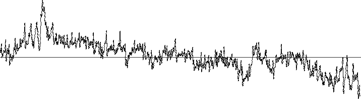
A 4 second sample of this signal is shown below
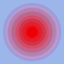
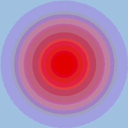
If one looks at the distribution of differences between samples, the graph looks as follows
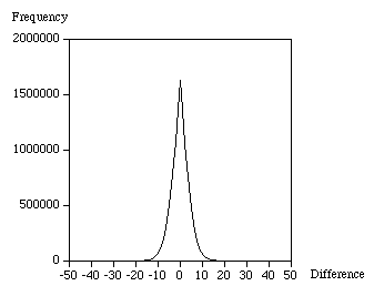
From this one might guess that 1 nibble (4 bits) should be used to represent differences between -7 and 7, 1 byte for differences between -127 and 127, and 2 bytes for the first sample and any larger differences. In each case the remaining sample in each range is used to flag a longer length for the next sample, for example negative 0 (1000) can be used as the flag for nibbles. For this example the number of differences stored as nibbles turned out to be 11739824, the number of items stored as bytes was 1098506, and finally there were only 6 differences that need 2 bytes. The file size from this simple minded delta coding is
This is a factor of 3.6 times smaller, the maximum saving if all the differences could be saved as nibbles would be 4.
There are lots of improvements that can be made to this, for example Huffman coding. The simplicity of this approach given the possible gains for many types of data from digitising signals in time makes it attractive for at least the initial data format. It is possible to measure the lowest number of bits needed theoretically to save a signal from Shannons information entropy measure. This is given by 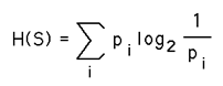
where pi is the probability of a particular symbol Si (number in this case) will occur in the sequence S.
RLE - Run Length EncodingWritten by Paul BourkeAugust 1995
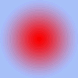
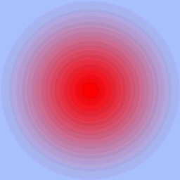
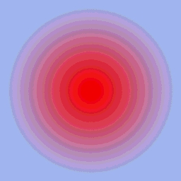
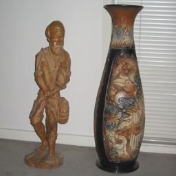
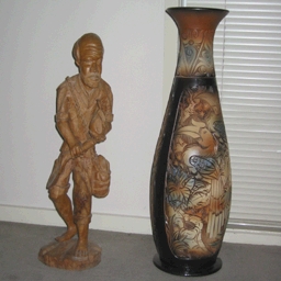
Introduction Run length encoding is a straightforward way of encoding data so that it takes up less space. It is relies on the string being encoded containing runs of the same character. Consider storing the following short string. abcddddddcbbbbabcdef There are 20 letters above, if each is stored as a single byte that is 20 bytes in all. However, the runs of "d" and "b' above can be stored as two bytes each, the first indicating how many letters in the run. For example, the following run length encoded string takes only 14 bytes. abc6dc4babcdef In general of course it needs to be a bit more sophisticated than the above. For example, there is no way in the above encoding to encode strings with numbers, that is, how would one know whether the number was the length of the run or part of the string content. Also, one would not want to encode runs of length 1 so how does one tell when a run starts and when a literal sequence starts. The common approach is to use only 7 of the 8 bits to indicate the run length, this is normally interpreted as a signed byte. If the length byte is positive it indicates a replicated run (run of the following byte). If the number is negative then it indicates a literal run, that is, that number of following bytes is copied as is. To illustrate this the following sequence of bytes would encode the example string given above, it requires 17 bytes. -3 a b c 6 d -1 c 4 b 6 a b c d e f While 17 bytes to encode what would take 20 without RLE may not sound like much, but as the frequency and length of the repeating characters increases the compression ratio gets better. Worst caseOf course RLE will not always result in a compression, consider a string where the next character is different from the current character. Every 127 bytes will require a extra byte to indicate a new literal run length. Best caseThe best case is when 128 identical characters follow each other, this is compressed into 2 bytes instead of 128 giving a compression ratio of 64. ExampleFor this reason RLE is most often used to compress black and white or 8 bit indexed colour images where long runs are likely. RLE compression is therefore what was used for the original low colour images expected for the Macintosh PICT file format. RLE is not generally used for high colour images such as photographs where in general each pixel will vary from the last. The following 3 images illustrate the different extremes, the first image contains runs along each row and will compress well. The second image is the same as the first but rotated 90 degrees so there are no runs giving worse case and a larger file. This suggests a natural extension to RLE for images, that is, one compresses vertically and horizontally and uses the best, the flag indicating which one is used is stored in the image header. The last case is the best scenario where the whole image is a constant value.
Image comparison
Run length encoding is used within a number of image formats, for example PNG, TIFF, and TGA. While RLE is normally used as a lossless compression, it can be assisted (to create small files) by quantising the rgb values thus increasing the chances of runs of the same colour. There are two ways one can run length encode the pixels, the first as used in the TGA format is to look for runs of all three components, the other is to compress each colour plane separately. The second approach normally gives smaller files. Below is a table for two different images along with the file size for the image quantised to different levels and saved in rgb order or planar order.
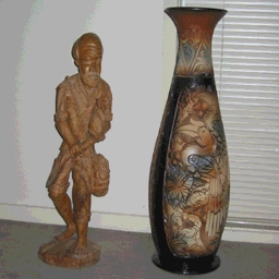
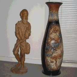
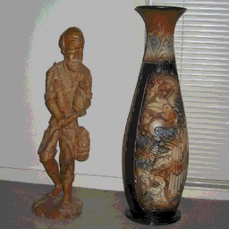
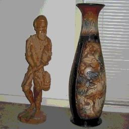
The above example was chosen because it doesn't have long runs of equal colour and because any banding due to quantisation should be obvious to spot. This occurs somewhere between 4 and 8 depending on how fussy one is. Note the planar compression works much better than the rgb based compression.
Unlike the first example, because each of the colour layers in this images are "busy" the difference between rgb and planar RLE compression is not so marked. Note that the visual artefacts that occur to so on the wall where there is a smooth and subtle shade variation, even at the highest quantisation level the artefacts on the vase are hard to pick. Source code
Standard compression C source: rle.c |